VERPAT Inputs and Parameters
VERPAT contains 5 definition files and 32 input files, some of which the user must change and others which typically remain unchanged. This page walks the end user through these files and specifies which files must be updated to implement VERPAT in a new region.
The following five files need to be configured in the "defs" directory:
The "run_parameters.json" file contains parameters that define key attributes of the model run and relationships to other model runs. A more detailed description of the file can be found here. The results of model run are stored in a directory with the name specified by "DatastoreName". This name should be changed when running different scenarios. For e.g. when running base scenario the output directory name can be set to BaseScenario by using "DatastoreName": ["BaseScenario"] in the file. The format of the VERPAT run_parameters.json file is as follows:
{
    "Model": ["RPAT"],
    "Scenario": ["RPAT Pilot"],
    "Description": ["Pilot RPAT module in VisionEval"],
    "Region": ["Multnomah County Oregon"],
    "BaseYear": ["2005"],
    "Years": ["2005", "2035"],
    "DatastoreName": ["Datastore"],
    "DatastoreType": ["RD"],
    "Seed": [1],
    "RunTypes": ["E", "ELESNP"]
}
Inputs Model Parameters Definitions
The "model_parameters.json" can contain global parameters for a particular model configuration that may be used by multiple modules. A more detailed description of the file and its structure can be found here. The description about the variables, required for VERPAT, listed in the file are documented by the modules that uses them in the inputs and outputs section. Some of these values may be modified to run scenarios. The variables that can be modified are described further Input Files. The format of the VERPAT model_parameters.json file is as follows:
[
  {"NAME": "EmploymentGrowth",
   "VALUE": "1.5",
   "TYPE": "double",
   "UNITS": "multiplier",
   "PROHIBIT": "",
   "ISELEMENTOF": ""},
  {
    "NAME": "FwyLaneMiGrowth",
    "VALUE": "1",
    "TYPE" : "double",
    "UNITS" : "multiplier",
    "PROHIBIT" : "c('NA', '< 0')",
    "ISELEMENTOF" : ""
  },
  {
    "NAME" : "ArtLaneMiGrowth",
    "VALUE": "1",
    "TYPE" : "double",
    "UNITS" : "multiplier",
    "PROHIBIT" : "c('NA', '< 0')",
    "ISELEMENTOF" : ""
  },
  .
  .
  .
  {
    "NAME" : "AutoCostGrowth",
    "VALUE": "1.5",
    "TYPE" : "double",
    "UNITS" : "multiplier",
    "PROHIBIT" : "c('NA', '< 0')",
    "ISELEMENTOF" : ""
  }
]
Inputs Model Parameters Definitions
The deflators.csv file defines the annual deflator values, such as the consumer price index, that are used to convert currency values between different years for currency denomination. This file does not need to be modified unless the years for which the dollar values used in the input dataset is not contained in this file. The format of the file is as follows:
| Year | Value |
|---|---|
| 1999 | 172.6 |
| 2000 | 178 |
| 2001 | 182.4 |
 |
|
Inputs Model Parameters Definitions
The "geography.csv" file describes all of the geographic relationships for the model and the names of geographic entities in a CSV-formatted text file. Azone, Bzone, and Marea should remain consistent with the input data. The format of the file is as follows:
| Azone | Bzone | Czone | Marea |
|---|---|---|---|
| Multnomah | Rur | NA | Multnomah |
| Multnomah | Sub_R | NA | Multnomah |
| Multnomah | Sub_E | NA | Multnomah |
| Multnomah | Sub_M | NA | Multnomah |
| Multnomah | Sub_T | NA | Multnomah |
| Multnomah | CIC_R | NA | Multnomah |
| Multnomah | CIC_E | NA | Multnomah |
| Multnomah | CIC_M | NA | Multnomah |
| Multnomah | CIC_T | NA | Multnomah |
| Multnomah | UC_R | NA | Multnomah |
| Multnomah | UC_E | NA | Multnomah |
| Multnomah | UC_M | NA | Multnomah |
| Multnomah | UC_T | NA | Multnomah |
The geography is described by 13 place types as shown below. One emerging school of thought in land use planning is to consider land uses in terms of place types instead of simply residential or commercial or high density compared to low density. A place type refers to all of the characteristics of a developed area including the types of uses included, the mix of uses, the density and intensity of uses.
| URBAN CORE |
CLOSE-IN COMMUNITY |
SUBURBAN | RURAL | |
|---|---|---|---|---|
| Residential |  |
|
|
|
| Commercial | |
|
|
|
| Mixed-Use | |
|
|
|
| Transit-Oriented Development | |
|
|
|
| Rural/Greenfield | |
An initial typology or system to organize place types can be traced to the Smart Growth Transect, which contained six zones in its original configuration including:
- Rural Preserve
- Rural Reserve
- Edge
- General
- Center
- Core
This approach to classifying place types was further refined in the Caltrans Smart Mobility which defined the following seven place types including:
- Urban Centers
- Close-In Compact Communities
- Compact Communities
- Suburban Communities
- Rural and Agricultural Lands
- Protected Lands
- Special Use Areas
Several of these place type categories provided additional options such as the Close-In Compact Communities which had three sub-definitions including Close-In-Centers, Close-In Corridors, and Close-In Neighborhoods.
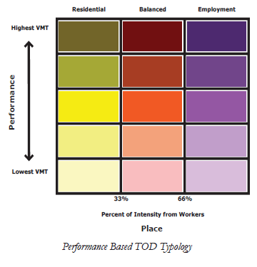
An alternative view of place types was provided by Reconnecting America, which developed a performance based place type approach for describing areas proximate to transit stations. Station areas would vary in terms of their relative focus between residential units, employees or a mix of the two. Station areas are also characterized on their relative intensity as well as shown below.
The approach employed for the place types in RPAT is therefore an amalgam of these approaches, in that the terminology is borrowed from the Smart Growth Transect and Caltrans Smart Mobility Study, while the relative performance of each place type is taken from the Reconnecting America approach but applied to a region instead of transit station sites.
Four general area types are defined in RPAT including:
- The Urban Core is the high-density mixed-use places with high jobs-housing ratios, well connected streets and high levels of pedestrian activities. It is anticipated that for many regions, the Urban Core will be the traditional downtown area of which there likely would be only one.
- The Close-in Community would be those areas located near to the Urban Cores and would consist primarily of housing with scattered mixed-use centers and arterial corridors. Housing would be varied in terms of density and type. Transit would be available with a primary focus on commute trips. These areas may be classified by their residents as suburban would be considered to be close-in communities given their adjacency to the Downtown and therefore the higher levels of regional accessibility.
- The Suburban place type is anticipated to represent the majority of development within regions. These communities are characterized by low level of integration of housing with jobs, retail, and services, poorly connected street networks, low levels of transit service, large amounts of surface parking, and limited walk ability.
- The Rural place type is defined as settlements of widely spaced towns separated by firms, vineyards, orchards, or grazing lands. These areas would be characterized by widely dispersed residential uses, little or no transit service, and very limited pedestrian facilities.
Further definition of the place types is allowed through the use of development types within the Urban Core, Close-in Community, and Suburban area types including:
- Residential includes all place types that are predominantly residential in character with limited employment and retail opportunities. Examples of this development type might include typical Suburban Residential or areas of the Downtown which are primarily residential as well. It is anticipated that this development type may be found in all of the area types except for rural.
- Employment includes those areas which are focused on employment with limited retail and residential. An example of this might include a Suburban Office Complex or a large cluster of office buildings within a Close-in Community or Urban Core. As with the residential development type, it is anticipated that this type of use would be found in all place types except for rural.
- Mixed-Use are those areas within a region which have a mix of residential, employment, and retail uses. While this development type can be found in the Suburban place type, it is most commonly found in the close-in community and urban core place type. Downtown areas that have retained their residential population to complement the employment are examples of this development type.
- Transit-Oriented Development (TOD) which is similar to the other development types in that it is applied to all area types except for Rural areas since it is thought to be highly unlikely that a rural TOD would be developed. The TOD development type is characterized by greater access to transit in all area types. Examples of this development type might include a Suburban TOD focused on a commuter rail station.
The process of allocating existing land use to the 13 place types is somewhat dependent on the types of data available in a region that describe existing land use, and the process can be either very detailed or somewhat simplified. The following description relays the process developed by Atlanta Regional Commission (ARC) as part of the pilot testing of RPAT and provides an example of how, mechanically, an agency can approach this allocation. It should be noted that this is merely one approach and not a specific recommendation for a method that should be followed.
In general, ARC followed a somewhat detailed process to derive input data from land use data as presented in their “Unified Growth Policy Map”, and from their regional travel demand model. They developed heuristics to align their land use with the 13 place types that RPAT uses.
The conversion of land use data to the place type scheme used in RPAT involved taking ARC’s Unified Growth Policy Map (UGPM) Areas and converting them to the 13 RPAT place types.
- The first step was to allocate the UGPM areas to the four area types used in RPAT. The Urban Core area type includes Region Core, Region Employment Centers and Aerotropolis UGPM areas; Close-in Community includes Maturing Neighborhoods; Suburban includes Developing Suburbs and Established Suburbs; and Rural includes Rural Areas and Developing Rural.
- The ARC traffic analysis zone (TAZ) system was overlaid with the area types and the centroid of the TAZ was used to determine its area type.
- The RPAT development type, the other dimension of the place type matrix, which included residential, mixed-use, employment, and TOD development types was determined for each TAZ not in the rural area type using the base year percentage of the TAZ’s employment in relation to the total of the population and employment in the TAZ. The mix between the employment and employment was used to determine the TAZs development type using the following cut points:
- Residential: < 33.33%
- Mixed Use: 33.33% to 66.67%
- Employment: > 66.67%
- Identify any TAZs that are TOD based on transit service and specific development types: only one TAZ was determined to be TOD as a development type, Lindbergh Center, in the Urban Core area type.
- The combination of the area type and the development type was then used to allocate all TAZs to one of the 13 place types.
The following is an enumeration of each place type abbreviation as it appears in the input file as well as a brief description of that value:
| Abbreviation | Description |
|---|---|
| Rur | Rural |
| Sub_R | Suburban Residential |
| Sub_E | Suburban Employment (i.e. Commercial) |
| Sub_M | Suburban Mixed Use |
| Sub_T | Suburban Transit Oriented Development |
| CIC_R | Close-in Community Residential |
| CIC_E | Close-in Community Employment (i.e. Commercial) |
| CIC_M | Close-in Community Mixed Use |
| CIC_T | Close-in Community Transit Oriented Development |
| UC_R | Urban Core Residential |
| UC_E | Urban Core Employment (i.e. Commercial) |
| UC_M | Urban Core Mixed Use |
| UC_T | Urban Core Transit Oriented Development |
Inputs Model Parameters Definitions
The "units.csv" file describes the default units to be used for storing complex data types in the model. This file should not be modified by the user. The format of the file is as follows:
| Type | Units |
|---|---|
| currency | USD |
| distance | MI |
| area | SQMI |
|
|
The VisionEval model system keeps track of the types and units of measure of all data that is processed. More details about the file and structure can be found here.
Inputs Model Parameters Definitions
The scenario inputs are split into four (4) categories: Built Environment, Demand, Policy, and Supply. There are two ways to specify these inputs. CSV Inputs are specified in a *.csv file and JSON Inputs are specified in model_parameters.json file. The users are encouraged to change these inputs to build different scenarios. The RPAT to VERPAT the connection between RPAT inputs to VERPAT inputs.
- CSV Inputs
- CSV Inputs
- JSON Inputs
- CSV Inputs
- CSV Inputs
- JSON Inputs
There are two ways to specify model parameters. CSV Parameters are specified in a *.csv file and JSON Parameters in a model_parameters.json file. While you are provided access to the model parameters, you are encouraged to use the default parameter values unless directed to use alternatives. Editing modeling parameters should be based only on research pertaining to local data sources and may result in unpredictable results.
- CSV Parameters
- model_accident_rates.csv
- model_fuel_prop_by_veh.csv
- model_fuel_composition_prop.csv
- model_fuel_co2.csv
- model_place_type_elasticities.csv
- model_place_type_relative_values.csv
- model_tdm_ridesharing.csv
- model_tdm_transit.csv
- model_tdm_transitlevels.csv
- model_tdm_vanpooling.csv
- model_tdm_workschedule.csv
- model_tdm_workschedulelevels.csv
- model_transportation_costs.csv
- model_veh_mpg_by_year.csv
- model_phev_range_prop_mpg_mpkwh.csv
- model_hev_prop_mpg.csv
- model_ev_range_prop_mpkwh.csv
- JSON Parameters
The user should change the input files described here.
Population and Jobs by Place Type: This file contains the distribution of population and employment among the 13 place types for base and future year. See this explanation for more infomation regarding place types. Each column, for each year, must sum to one (1). It is acceptable to have no land use (i.e. a value of 0) in certain categories.
The yearly TAZ employment and population totals were summed by the 13 place type and then scaled to total one for both employment and population. The allocation of growth between the base and the future years in population and employment to each of the 13 place types is captured by the rows containing future years. The discussion of the population and jobs by place type input above describes how to allocate existing land use to the 13 place types. A similar approach can be used to allocate expected growth from spatial planning resources such as TAZ or Census Block Group level forecasts to the place types. Here is a snapshot of the file:
| Geo | Year | Pop | Emp |
|---|---|---|---|
| Rur | 2005 | 0.05 | 0.1 |
| Sub_R | 2005 | 0.3 | 0 |
| Sub_E | 2005 | 0 | 0.2 |
| Sub_M | 2005 | 0.1 | 0.1 |
| Sub_T | 2005 | 0 | 0 |
| CIC_R | 2005 | 0.15 | 0 |
| CIC_E | 2005 | 0 | 0.2 |
| CIC_M | 2005 | 0.1 | 0.1 |
| CIC_T | 2005 | 0 | 0 |
| UC_R | 2005 | 0.1 | 0 |
| UC_E | 2005 | 0 | 0.1 |
| UC_M | 2005 | 0.1 | 0.1 |
| UC_T | 2005 | 0.1 | 0.1 |
| Rur | 2035 | 0.05 | 0.1 |
| Sub_R | 2035 | 0.3 | 0 |
| Sub_E | 2035 | 0 | 0.2 |
| Sub_M | 2035 | 0.1 | 0.1 |
| Sub_T | 2035 | 0 | 0 |
| CIC_R | 2035 | 0.15 | 0 |
| CIC_E | 2035 | 0 | 0.2 |
| CIC_M | 2035 | 0.1 | 0.1 |
| CIC_T | 2035 | 0 | 0 |
| UC_R | 2035 | 0.1 | 0 |
| UC_E | 2035 | 0 | 0.1 |
| UC_M | 2035 | 0.1 | 0.1 |
| UC_T | 2035 | 0.1 | 0.1 |
Inputs Model Parameters Definitions
Auto and transit trips per capita: This file contains regional averages for auto and transit trips per capita per day for the base year.
- Auto is the regional average of auto trips per capita, including drive alone and shared ride travel. This data can be derived from the National Household Travel Survey by region or from a local household travel survey or regional travel demand forecasting model.
- Transit is the regional average of transit trips per capita, including walk and drive access to transit. This data can be derived from the National Transit Database where the annual database contains a “service” table that has annual transit trip data for each transit operator or from a local household travel survey or regional travel demand forecasting model.
Here is a snapshot of the files:
| Mode | Trips |
|---|---|
| Auto | 3.2 |
| Transit | 0.4 |
Inputs Model Parameters Definitions
Employment: This file contains employment data for each of the counties that make up the region. The file is derived from County Business Pattern (CBP) data by county. Industries are categorized by the North American Industrial Classification System (NAICS) 6 digit codes. Firm size categories are:
- n1_4: 1- 4 employees
- n5_9: 5-9 employees
- n10_19: 10-19 employees
- n20_99: 20-99 employees
- n100_249: 100-249 employees
- n250_499: 250-499 employees
- n500_999: 500-999 employees
- n1000: 1,000 or More Employee Size Class
- n1000_1: 1,000-1,499 employees
- n1000_2: 1,500-2,499 employees
- n1000_3: 2,500 to 4, 999 Employees
- n1000_4: Over 5,000 employees
While the county field is required to be present, the business synthesis process does not require a meaningful value and therefore users may simply enter 'region'. The consistency in the naming of the "region" should be maintained across all the files that contains the label "county" or "Geo". It is also not necessary to use such detailed NAICS categories if those are not available; the current business synthesis model and subsequent models do not use this level of detail (although future versions of the model may) – at minimum, the number of establishments for all employment types can be provided by size category. Regions with significant employment in industries such as government and public administration that are not covered by the CBP may need to add records to the file that cover this type of employment to more accurately match employment totals in their region. The two additional fields contained in the file are:
- emp: Total number of employees
- est: Total number of establishments
Here is the snapshot of the file:
| county | year | naics | emp | est | n1_4 | n5_9 | n10_19 | n20_49 | n50_99 | n100_249 | n250_499 | n500_999 | n1000 | n1000_1 | n1000_2 | n1000_3 | n1000_4 |
|---|---|---|---|---|---|---|---|---|---|---|---|---|---|---|---|---|---|
| Multnomah | 2005 | 113110 | 0 | 5 | 2 | 1 | 0 | 2 | 0 | 0 | 0 | 0 | 0 | 0 | 0 | 0 | 0 |
| Multnomah | 2005 | 113310 | 0 | 3 | 2 | 0 | 0 | 1 | 0 | 0 | 0 | 0 | 0 | 0 | 0 | 0 | 0 |
| Multnomah | 2005 | 114111 | 0 | 1 | 0 | 1 | 0 | 0 | 0 | 0 | 0 | 0 | 0 | 0 | 0 | 0 | 0 |
| Multnomah | 2005 | 114112 | 0 | 1 | 1 | 0 | 0 | 0 | 0 | 0 | 0 | 0 | 0 | 0 | 0 | 0 | 0 |
| Multnomah | 2005 | 115114 | 0 | 1 | 0 | 0 | 0 | 0 | 0 | 0 | 1 | 0 | 0 | 0 | 0 | 0 | 0 |
| Multnomah | 2005 | 115210 | 0 | 4 | 3 | 1 | 0 | 0 | 0 | 0 | 0 | 0 | 0 | 0 | 0 | 0 | 0 |
| Multnomah | 2005 | 115310 | 0 | 5 | 2 | 0 | 1 | 1 | 1 | 0 | 0 | 0 | 0 | 0 | 0 | 0 | 0 |
| Multnomah | 2005 | 212319 | 0 | 1 | 1 | 0 | 0 | 0 | 0 | 0 | 0 | 0 | 0 | 0 | 0 | 0 | 0 |
| Multnomah | 2005 | 212321 | 0 | 4 | 1 | 1 | 1 | 1 | 0 | 0 | 0 | 0 | 0 | 0 | 0 | 0 | 0 |
Inputs Model Parameters Definitions
Household population: This file contains population estimates/forecasts by county and age cohort for each of the base and future years. The file format includes six age categories used by the population synthesis model:
- 0-14
- 15-19
- 20-29
- 30-54
- 55-64
- 65 Plus
Future year data must be developed by the user; in many regions population forecasts are available from regional or state agencies and/or local academic sources. As with the employment data inputs the future data need not be county specific. Rather, regional totals by age group can be entered into the file with a value such as “region” entered in the county field.
Here is a snapshot of the file:
| Geo | Year | Age0to14 | Age15to19 | Age20to29 | Age30to54 | Age55to64 | Age65Plus |
|---|---|---|---|---|---|---|---|
| Multnomah | 2005 | 129869 | 41133 | 99664 | 277854 | 71658 | 72648 |
| Multnomah | 2035 | 169200 | 48800 | 144050 | 327750 | 116100 | 162800 |
Inputs Model Parameters Definitions
Group quarter population: This file contains group quarters population estimates/forecasts by county and age cohort for each of the base and future years. The file format includes six age categories used by the population synthesis model:
- 0-14
- 15-19
- 20-29
- 30-54
- 55-64
- 65 Plus
Here is a snapshot of the file:
| Geo | Year | GrpAge0to14 | GrpAge15to19 | GrpAge20to29 | GrpAge30to54 | GrpAge55to64 | GrpAge65Plus |
|---|---|---|---|---|---|---|---|
| Multnomah | 2005 | 0 | 0 | 0 | 1 | 0 | 0 |
| Multnomah | 2035 | 0 | 0 | 0 | 1 | 0 | 0 |
Inputs Model Parameters Definitions
Household size (azone_hhsize_targets.csv): This file contains the household specific targets. This contain two household specific attributes:
- AveHhSize: Average household size of households (non-group quarters)
- Prop1PerHh: Proportion of households (non-group quarters) having only one person
Here is a snapshot of the file:
| Geo | Year | AveHhSize | Prop1PerHh |
|---|---|---|---|
| Multnomah | 2005 | NA | NA |
| Multnomah | 2035 | NA | NA |
Inputs Model Parameters Definitions
Regional income: This file contains information on regional average per capita household (HHIncomePC) and group quarters (GQIncomePC) income by forecast year in year 2000 dollars. The data can be obtained from the U.S. Department of Commerce Bureau of Economic Analysis for the current year or from regional or state sources for forecast years. In order to use current year dollars just replace 2000 in column labels with current year. For example, if the data is obtained in year 2005 dollars then the column labels in the file shown below will become HHIncomePC.2005 and GQIncomePC.2005. Here is a snapshot of the file:
| Geo | Year | HHIncomePC.2000 | GQIncomePC.2000 |
|---|---|---|---|
| Multnomah | 2005 | 32515 | 0 |
| Multnomah | 2035 | 40000 | 0 |
Inputs Model Parameters Definitions
Relative employment: This file contains ratio of workers to persons by age cohort in model year vs. estimation data year. The relative employment value for each age group, which is the employment rate for the age group relative to the employment rate for the model estimation year data is used to adjust the relative employment to reflect changes in relative employment for other years. This file contains five age cohorts:
- RelEmp15to19: Ratio of workers to persons age 15 to 19 in model year vs. in estimation data year
- RelEmp20to29: Ratio of workers to persons age 20 to 29 in model year vs. in estimation data year
- RelEmp30to54: Ratio of workers to persons age 30 to 54 in model year vs. in estimation data year
- RelEmp55to64: Ratio of workers to persons age 55 to 64 in model year vs. in estimation data year
- RelEmp65Plus: Ratio of workers to persons age 65 or older in model year vs. in estimation data year
Here is a snapshot of the file:
| Geo | Year | RelEmp15to19 | RelEmp20to29 | RelEmp30to54 | RelEmp55to64 | RelEmp65Plus |
|---|---|---|---|---|---|---|
| Multnomah | 2005 | 1 | 1 | 1 | 1 | 1 |
| Multnomah | 2035 | 1 | 1 | 1 | 1 | 1 |
Inputs Model Parameters Definitions
Truck and bus vmt: This file contains the region’s proportion of VMT by truck and bus as well as the distribution of that VMT across functional classes (freeway, arterial, other). The file includes one row for bus VMT data and one row for Truck VMT data. It should be noted that it is not necessary to enter values in the PropVmt column for BusVmt as this is calculated using the values in the transportation_supply.csv #EDIT (marea_rev_miles_pc.csv?) user input file. The truck VMT proportion (PropVMT column, TruckVMT row) can be obtained from Highway Performance Monitoring System data and local sources or the regional travel demand model if one exists. The proportions of VMT by functional class can be derived from the Federal Highway Cost Allocation Study and data from transit operators. The Federal Highway Cost Allocation Study (Table II-6, 1997 Federal Highway Cost Allocation Study Final Report, Chapter II is used to calculate the average proportion of truck VMT by functional class. Data from transit authorities are used to calculate the proportions of bus VMT by urban area functional class. Here is a snapshot of the file:
| Type | PropVmt | Fwy | Art | Other |
|---|---|---|---|---|
| BusVmt | 0 | 0.15 | 0.591854 | 0.258146 |
| TruckVmt | 0.08 | 0.452028 | 0.398645 | 0.149327 |
Inputs Model Parameters Definitions
Light vehicle dvmt (BaseLtVehDvmt): Total light vehicle daily VMT for the base year in thousands of miles. This data can be derived from a combination of Highway Performance Monitoring System data, Federal Highway Cost Allocation Study data, and regional data. Light vehicle daily VMT can be estimated by subtracting truck and bus VMT from total VMT provided in the Highway Performance Monitoring System (HPMS). Regional travel demand model outputs can also be used to derive these data. It should be defined in model_parameters.json as follows:
{
    "NAME" : "BaseLtVehDvmt",
    "VALUE": "27244",
    "TYPE" : "compound",
    "UNITS" : "MI/DAY",
    "PROHIBIT" : "c('NA', '< 0')",
    "ISELEMENTOF" : ""
}
Inputs Model Parameters Definitions
Dvmt proportion by functional class (BaseFwyArtProp): The proportions of daily VMT for light vehicles that takes place on freeways and arterials (i.e., the remainder of VMT takes place on lower functional class roads for the base year. This data can be derived from a combination of Highway Performance Monitoring System data, Federal Highway Cost Allocation Study data, and regional data. The proportions of light vehicle daily VMT on freeways and arterials can be derived from the HPMS data. Regional travel demand model outputs can also be used to derive these data. It should be defined in model_parameters.json as follows:
{
    "NAME" : "BaseFwyArtProp",
    "VALUE": "0.77",
    "TYPE" : "double",
    "UNITS" : "proportion",
    "PROHIBIT" : "c('NA', '< 0', '> 1')",
    "ISELEMENTOF" : ""
}
Inputs Model Parameters Definitions
Employment Growth (EmploymentGrowth): This variable represents a growth rate for employment in the region between the base year and the future year. A rate of 1 indicates no changes in overall employment, a value of more than 1 indicates some growth (e.g., 1.5 = 50% growth) and a value of less than 1 indicates decline in employment. It should be defined in model_parameters.json as follows:
{
    "NAME": "EmploymentGrowth",
    "VALUE": "1.5",
    "TYPE": "double",
    "UNITS": "multiplier",
    "PROHIBIT": "",
    "ISELEMENTOF": ""
}
Inputs Model Parameters Definitions
Road lane miles: This file contains the amount of transportation supply by base year in terms of lane miles of freeways and arterial roadways in the region. The base year data is duplicated for future year. Freeway and Arterial are total lane miles for those functional classes in the region. These data can be derived from the Federal Highway Administration’s (FHWA) Highway Statistics data. Here is a snapshot of the file:
| Geo | Year | FwyLaneMi | ArtLaneMi |
|---|---|---|---|
| Multnomah | 2005 | 250 | 900 |
| Multnomah | 2035 | 250 | 900 |
Inputs Model Parameters Definitions
Transit revenue miles: This file contains the amount of transportation supply by base year in terms of the revenue miles operating by the transit system in the region. The base year data is duplicated for future year. Bus and Rail are annual bus and rail revenue miles per capita for the region. These data can be derived from the National Transit Database, where the annual database contains a “service” table that has annual revenue mile data by mode for each transit operator. Here is a snapshot of the file:
| Geo | Year | BusRevMiPC | RailRevMiPC |
|---|---|---|---|
| Multnomah | 2005 | 19 | 4 |
| Multnomah | 2035 | 19 | 4 |
Inputs Model Parameters Definitions
Percentage of employees offered commute options: This file contains assumptions about the availability and participation in work based travel demand management programs. The policies are ridesharing programs, transit pass programs, telecommuting or alternative work schedule programs, and vanpool programs. For each, the user enters the proportion of workers who participate (the data items with the “Participation” suffix). For one program, the transit subsidy, the user must also enter the subsidy level in dollars for the TransitSubsidyLevel data item. Here is a snapshot of the file:
| TDMProgram | DataItem | DataValue |
|---|---|---|
| Ridesharing | RidesharingParticipation | 0.05 |
| TransitSubsidy | TransitSubsidyParticipation | 0.1 |
| TransitSubsidy | TransitSubsidyLevel | 1.25 |
| WorkSchedule | Schedule980Participation | 0.01 |
| WorkSchedule | Schedule440Participation | 0.01 |
| WorkSchedule | Telecommute1.5DaysParticipation | 0.01 |
| Vanpooling | LowLevelParticipation | 0.04 |
| Vanpooling | MediumLevelParticipation | 0.01 |
| Vanpooling | HighLevelParticipation | 0.01 |
Inputs Model Parameters Definitions
Percent road miles with ITS treatment: This file is an estimate of the proportion of road miles that have improvements which reduce incidents through ITS treatments in both the base and future years. Values entered should be between 0 and 1, with 1 indicating that 100% of road miles are treated. The ITS policy measures the effects of incident management supported by ITS. The ITS table is used to inform the congestion model and the travel demand model. The model uses the mean speeds with and without incidents to compute an overall average speed by road type and congestion level providing a simple level of sensitivity to the potential effects of incident management programs on delay and emissions. The ITS treatments are evaluated only on freeways and arterials. The ITS treatments that can be evaluated are those that the analyst considers will reduce non-recurring congestion due to incidents. This policy does not deal with other operational improvements such as signal coordination, or temporary capacity increases such as allowing shoulder use in the peak. Here is a snapshot of the file:
| Geo | Year | ITS |
|---|---|---|
| Multnomah | 2005 | 0 |
| Multnomah | 2035 | 0 |
Inputs Model Parameters Definitions
Bicycling/light vehicles targets: This file contains input data for the non-motorized vehicle model. In VERPAT, non-motorized vehicles are bicycles, and also electric bicycles, segways, and similar vehicles that are small, light-weight and can travel at bicycle speeds or slightly higher. The parameters are as follows:
- TargetProp: non-motorized vehicle ownership rate (average ratio of non-motorized vehicles to driver age population)
- Threshold: single-occupant vehicle (SOV) tour mileage threshold used in the SOV travel proportion model. This is the upper limit for tour lengths that are suitable for reallocation to non-motorized modes.
- PropSuitable: proportion of SOV travel suitable for non-motorized vehicle travel. This variable describes the proportion of SOV tours within the mileage threshold for which non-motorized vehicles might be substituted. This variable takes into account such factors as weather and trip purpose.
The non-motorized vehicle model predicts the ownership and use of non-motorized vehicles (where non-motorized vehicles are bicycles, and also electric bicycles, segways and similar vehicles that are small, light-weight and can travel at bicycle speeds or slightly higher than bicycle speeds). The core concept of the model is that non-motorized vehicle usage will primarily be a substitute for short-distance SOV travel. Therefore, the model estimates the proportion of the household vehicle travel that occurs in short-distance SOV tours. The model determines the maximum potential for household VMT to be diverted to non-motorized vehicles, which is also dependent on the availability of non-motorized vehicles. Note that bike share programs (BSP) serve to increase the availability of non-motorized vehicles and can be taken into account by increasing the TargetProp variable. Use national estimates of non-motorized ownership if regional estimates of non-motorized ownership are not available (unless the region has notably atypical levels of bicycle usage). See Bicycle Ownership in the United States for an analysis of regional differences. Here is a snapshot of the file:
| DataItem | DataValue |
|---|---|
| TargetProp | 0.2 |
| Threshold | 2 |
| PropSuitable | 0.1 |
Inputs Model Parameters Definitions
Increase in parking cost and supply: This file contains information that allows the effects of policies such as workplace parking charges and "cash-out buy-back" programs to be tested. The input parameters are as follows and should be entered for both the base and future year:
- PropWorkParking: proportion of employees that park at work
- PropWorkCharged: proportion of employers that charge for parking
- PropCashOut: proportion of employment parking that is converted from being free to pay under a "cash-out buy-back" type of program
- PropOtherCharged: proportion of other parking that is not free
- ParkingCost.2000: average daily parking cost in 2000 year USD. In order to use base year dollars just replace 2000 in column labels with base year. This variable is the average daily parking cost for those who incur a fee to park. If the paid parking varies across the region, then the "PkgCost" value should reflect the average of those parking fees, but weighted by the supply – so if most parking is in the Center City, then the average will be heavily weighted toward the price in the Center City.
Here is a snapshot of the file:
| Geo | Year | PropWorkParking | PropWorkCharged | PropCashOut | PropOtherCharged | ParkingCost.2000 |
|---|---|---|---|---|---|---|
| Multnomah | 2005 | 1 | 0.1 | 0 | 0.05 | 5 |
| Multnomah | 2035 | 1 | 0.1 | 0 | 0.05 | 5 |
Inputs Model Parameters Definitions
% Increase in Auto Operating Cost (AutoCostGrowth): This parameter reflects the proportional increase in auto operating cost. This can be used to test different assumptions for future gas prices or the effects of increased gas taxes. A value of 1.5 multiplies base year operating costs by 1.5 and thus reflects a 50% increase. It should be defined in model_parameters.json as follows:
{
    "NAME" : "AutoCostGrowth",
    "VALUE": "1.5",
    "TYPE" : "double",
    "UNITS" : "multiplier",
    "PROHIBIT" : "c('NA', '< 0')",
    "ISELEMENTOF" : ""
}
Inputs Model Parameters Definitions
FwyLaneMiGrowth: The variable indicates the percent increase in supply of freeways lane miles in the future year compared to base year. By default, the transportation supply is assumed to grow in line with population increase; therefore a value of 1 indicates growth in proportion with population growth. A value less than 1 indicates that there will be less freeway lane mile supply, per person, in the future. A value of 1 indicates faster freeway expansion than population growth. It should be defined in model_parameters.json as follows:
{
    "NAME": "FwyLaneMiGrowth",
    "VALUE": "1",
    "TYPE" : "double",
    "UNITS" : "multiplier",
    "PROHIBIT" : "c('NA', '< 0')",
    "ISELEMENTOF" : ""
}
Inputs Model Parameters Definitions
ArtLaneMiGrowth: The variable indicates the percent increase in supply of arterial lane miles in the future year compared to base year. It is a similar value to freeway except that it measures arterial lane mile growth. It is also proportional to population growth. It should be defined in model_parameters.json as follows:
{
    "NAME" : "ArtLaneMiGrowth",
    "VALUE": "1",
    "TYPE" : "double",
    "UNITS" : "multiplier",
    "PROHIBIT" : "c('NA', '< 0')",
    "ISELEMENTOF" : ""
}
Inputs Model Parameters Definitions
BusRevMiPCGrowth: It is the percent increase in transit revenue miles per capita for bus. It behaves in a similar way to the freeway and rail values in that a value of 1 indicates per capita revenue miles stays constant. It should be defined in model_parameters.json as follows:
{
    "NAME" : "BusRevMiPCGrowth",
    "VALUE": "1",
    "TYPE" : "double",
    "UNITS" : "multiplier",
    "PROHIBIT" : "c('NA', '< 0')",
    "ISELEMENTOF" : ""
}
Inputs Model Parameters Definitions
RailRevMiPCGrowth: It is the percent increase in transit revenue miles per capita for rail. This encompasses all rail modes, from light rail through to commuter rail. It should be defined in model_parameters.json as follows:
{
    "NAME" : "RailRevMiPCGrowth",
    "VALUE": "1",
    "TYPE" : "double",
    "UNITS" : "multiplier",
    "PROHIBIT" : "c('NA', '< 0')",
    "ISELEMENTOF" : ""
}
Inputs Model Parameters Definitions
Auto Operating Surcharge Per VMT (VmtCharge): It is a cost in cents per mile that would be levied on auto users through the form of a VMT charge. It should be defined in model_parameters.json as follows:
{
    "NAME" : "VmtCharge",
    "VALUE": "0.05",
    "TYPE" : "compound",
    "UNITS" : "USD/MI",
    "PROHIBIT" : "c('NA', '< 0')",
    "ISELEMENTOF" : ""
}
Inputs Model Parameters Definitions
Users can modify these parameters to test alternative scenarios. For e.g. users can use model_veh_mpg_by_year.csv to test alternative vehicle development scenarios, such as improved technology and/or fuel economy standards that lead to higher fuel economies.
Accident Rates: Road safety impacts are calculated by factoring the amount of VMT. The following national average rates, from the Fatality Analysis Reporting System General Estimates System (2009) by US Department of Transportation, are applied to calculate the number of fatal and injury accidents and the value of property damage:
- Fatal: 1.14 per 100 Million Miles Traveled
- Injury: 51.35 per 100 Million Miles Traveled
- Property damage: 133.95 per 100 Million Miles Traveled
Here is a snapshot of the file:
| Accident | Rate |
|---|---|
| Fatal | 1.14 |
| Injury | 51.35 |
| Property | 133.95 |
Inputs Model Parameters Definitions
Vehicle VMT proportion by fuel (model_fuel_prop_by_veh.csv): The file contains allocation of VMT for each of the four road vehicle types that VERPAT represents (auto, light truck, bus, and heavy truck) to different fuel types (Diesel, CNG, Gasoline). This file is used in the calculations of fuel consumption. This file can be used to test alternative fuel scenarios by varying the shares of non-gasoline fuels.
- PropDiesel: The proportion of the fleet that uses diesel
- PropCng: The proportion of the fleet that uses CNG
- PropGas: The proportion of the fleet that uses gasoline
Here is a snapshot of the file:
| VehType | PropDiesel | PropCng | PropGas |
|---|---|---|---|
| Auto | 0.007 | 0 | 0.993 |
| LtTruck | 0.04 | 0 | 0.96 |
| Bus | 0.995 | 0.005 | 0 |
| Truck | 0.945 | 0.005 | 0.05 |
Inputs Model Parameters Definitions
Fuel composition: This file contains the composition of fuel used for each of the four road vehicle types that VERPAT represents (auto, light truck, bus, and heavy truck). This file is also used in the calculations of fuel consumption along with the aforementioned file. The column labels in the file are:
- GasPropEth: The average ethanol proportion in gasoline sold
- DieselPropBio: The average biodiesel proportion in diesel sold
Here is a snapshot of the file:
| VehType | GasPropEth | DieselPropBio |
|---|---|---|
| Auto | 0.1 | 0.05 |
| LtTruck | 0.1 | 0.05 |
| Bus | 0.1 | 0.05 |
| Truck | 0.1 | 0.01 |
Inputs Model Parameters Definitions
Emission Rate: The emissions rate file contains information on “pump-to-wheels” CO2 equivalent emissions by fuel type in grams per mega Joule of fuel energy content. There is one row for each fuel type: ULSD, biodiesel, RFG (reformulated gasoline), CARBOB (gasoline formulated to be blended with ethanol), ethanol, and CNG. This file is used to convert fuel use to CO2 equivalent emissions. Here is a snapshot of the file:
| Fuel | Intensity |
|---|---|
| ULSD | 77.19 |
| Biodiesel | 76.81 |
| RFG | 75.65 |
| CARBOB | 75.65 |
| Ethanol | 74.88 |
| Cng | 62.14 |
Inputs Model Parameters Definitions
This file contains elasticities for four performance metrics:
- VMT – Following the estimate of travel demand that incorporates induced demand, an adjustment is made to travel demand that accounts for changes in growth by the place types that are used in the model to describe urban form. These changes are interpreted as changes in design (intersection street density), accessibility (job accessibility by auto), distance to transit (nearest transit stop), density (population density) and diversity (land use mix). The effect on travel demand is determined as changes in VMT by these urban form categories, as shown in the table below. The elasticities that are shown in the table are multiplied by the D values for each place type. The D values are proportion values for each place type that are relative to the regional average, which is set to 1.0.
- VehicleTrips – The change in the number of vehicle trips is calculated using a set of elasticities from Index 4D Values (2001) that pivots from the current number of vehicle trips per capita based on the scenario’s allocation of growth by place type. The elasticities shown in the table are applied to D values, which are proportional values for each place type that are relative to a regional average for that D value that is set to 1.0. The model reports the additional number of trips caused by the growth assumed in the scenario and not the regional total.
- TransitTrips – The change in the number of transit trips is calculated using a set of elasticities from Index 4D Values (2001) that pivots from the current number of transit trips per capita based on the scenario’s allocation of growth by place type. The elasticities shown in the table are applied to D values, which are proportional values for each place type that are relative to a regional average for that D value that is set to 1.0. The model reports the additional number of trips caused by the growth assumed in the scenario and not the regional total.
- Walking – The elasticities shown in the table are applied to D values, which are proportional values for each place type that are relative to a regional average for that D value that is set to 1.0. The product of the elasticity and D value is applied to the place type growth quantities for the scenario to calculated the percentage increase or decrease in walking for new residents in the region relative to a the current place type distribution.
Here is a snapshot of the file:
| Parameters | VMT | VehicleTrips | TransitTrips | Walking |
|---|---|---|---|---|
| Density | -0.04 | -0.043 | 0.07 | 0.07 |
| Diversity | -0.09 | -0.051 | 0.12 | 0.15 |
| Design | -0.12 | -0.031 | 0.23 | 0.39 |
| Regional_Accessibility | -0.2 | -0.036 | 0 | 0 |
| Distance_to_Transit | -0.05 | 0 | 0.29 | 0.15 |
Inputs Model Parameters Definitions
This file contains the D values, which are proportional values for each of the 13 place types (Bzones) that are relative to a regional average, for each of the five Ds used in VERPAT - design (intersection street density), accessibility (job accessibility by auto), distance to transit (nearest transit stop), density (population density) and diversity (land use mix). Here is a snapshot of the file:
| Geo | Density | Diversity | Design | Regional_Accessibility | Distance_to_Transit |
|---|---|---|---|---|---|
| Rur | 0.5 | 0.5 | 0.5 | 0.5 | 0.5 |
| Sub_R | 0.75 | 0.75 | 0.75 | 0.75 | 0.75 |
| Sub_E | 0.75 | 0.75 | 0.75 | 0.75 | 0.75 |
| Sub_M | 1 | 1 | 1 | 0.75 | 0.75 |
| Sub_T | 1 | 1 | 1 | 1 | 1 |
| CIC_R | 1.2 | 1.2 | 1.2 | 1.2 | 1 |
| CIC_E | 1.2 | 1.2 | 1.2 | 1.2 | 1 |
| CIC_M | 1.2 | 1.2 | 1.2 | 1.2 | 1 |
| CIC_T | 1.2 | 1.2 | 1.2 | 1.2 | 1.2 |
| UC_R | 1.5 | 1.2 | 1.5 | 1.5 | 1.2 |
| UC_E | 1.5 | 1.2 | 1.5 | 1.5 | 1.2 |
| UC_M | 1.5 | 1.5 | 1.5 | 1.5 | 1.2 |
| UC_T | 1.5 | 1.5 | 1.5 | 1.5 | 1.5 |
Inputs Model Parameters Definitions
Travel Demand Management: Ridesharing: The ridesharing Travel Demand Management file contains parameters describing the effectiveness of ridesharing programs by place type. The proportion of employees participating in the ridesharing program is a policy input. This is converted into a proportion of working-age persons by using an assumed labor force participation rate (0.65) to sample working-age persons in households. The ridesharing sub-model then computes the anticipated level of VMT reduction resulting from the implementation of ridesharing, based on the place type the household lives in, using the effectiveness values shown in this parameter file. Previous studies have determined that the level of ridesharing participation will be less in the rural and suburban areas, as compared to the more-urban areas. Typically, more people will carpool in the more urbanized areas due to the presence of parking charges, potential difficulties in finding parking, and other disincentives that are typically present in more urbanized areas. Here is a snapshot of the file:
| ModelGeo | Effectiveness |
|---|---|
| Rur | 0 |
| Sub | 0.05 |
| CIC | 0.1 |
| UC | 0.15 |
Inputs Model Parameters Definitions
Travel Demand Management: Transit Fares: The transit fare Travel Demand Management files are parameters for the effectiveness (level of VMT reduction) and fare subsidy values for employer. The subsidized/discounted transit model begins by evaluating the level of participation within the region. Monte Carlo processes are used to identify which households participate in transit pass programs. The proportion of employees participating in this program is a policy input. This is converted into a proportion of working-age persons by using an assumed labor force participation rate (0.65) to sample working-age persons in households. The model then allows the selection of one of four potential subsidy levels (also a policy inputs), which influence the level of VMT reduction based on the level of subsidy applied to the place type. The anticipated level of VMT reduction is then further reduced to account for the proportion of work travel in overall daily travel. Here is a snapshot of the file:
| ModelGeo | Subsidy0 | Subsidy1 | Subsidy2 | Subsidy3 | Subsidy4 |
|---|---|---|---|---|---|
| Rur | 0 | 0 | 0 | 0 | 0 |
| Sub | 0 | 0.02 | 0.033 | 0.079 | 0.2 |
| CIC | 0 | 0.034 | 0.073 | 0.164 | 0.2 |
| UC | 0 | 0.062 | 0.129 | 0.2 | 0.2 |
Inputs Model Parameters Definitions
Travel Demand Management: Transit Subsidy Levels: This file contains the dollar value match to the subsidy levels used in model_tdm_transit.csv file. Here is a snapshot of the file:
| SubsidyLevel | SubsidyValue.2000 |
|---|---|
| Subsidy0 | 0 |
| Subsidy1 | 0.75 |
| Subsidy2 | 1.49 |
| Subsidy3 | 2.98 |
| Subsidy4 | 5.96 |
Inputs Model Parameters Definitions
Travel Demand Management: Vanpooling: This file contains parameters describing the effectiveness in terms of VMT reductions for vanpooling programs across three levels of employee involvement. The vanpool program sub-model operates by evaluating the likely level of participation. Monte Carlo processes are used to identify which households participate in vanpool programs. The proportion of employees participating in this program is a policy input. This is converted into a proportion of working-age persons by using an assumed labor force participation rate (0.65) to sample working-age persons in households. Those employers that would participate in the program are then categorized into three levels of involvement from low to medium to high. The level of involvement reflects the extent to which an employer would actively facilitate and promote vanpooling. For example, a low level of involvement might represent an employer who organizes only a minimal number of vanpools. The high level of involvement could represent an employer who has an extensive vanpooling program to cover a large number of employees. Based on the level of involvement, the reduction in VMT is estimated on the basis of the values in this file. Here is a snapshot of the file:
| VanpoolingParticipation | VMTReduction |
|---|---|
| Low | 0.003 |
| Medium | 0.0685 |
| High | 0.134 |
Inputs Model Parameters Definitions
Travel Demand Management: Work Schedule: This file contains parameters that describe the effectiveness for different participation levels for three different telecommuting or alternative work schedules. The telecommuting or alternative work schedule model first evaluates the likely level of participation throughout the region in terms of telecommuting or alternatively-works schedules. Monte Carlo processes are used to identify which households participate in telecommuting programs. The proportion of employees participating in this program is a policy input. This is converted into a proportion of working-age persons by using an assumed labor force participation rate (0.65) to sample working-age persons in households. The model then determines the type of programs that might be implemented. Three potential alternatives are offered including:
- 4/40 Schedule: 4 days per week with 40 hours per week
- 9/80 Schedule: working 4 days every other week with an average of 80 hours over 2 weeks
- Telecommuting: Workers may work 1 to 2 days a week remotely
Once the option has been identified and the level of participation, the estimated VMT is determined on the basis of the parameters in this file. Here is a snapshot of the file:
| WorkSchedulePolicy | Participation0 | Participation1 | Participation2 | Participation3 | Participation4 | Participation5 |
|---|---|---|---|---|---|---|
| Schedule980 | 0 | 0.0007 | 0.0021 | 0.0035 | 0.007 | 0.0175 |
| Schedule440 | 0 | 0.0015 | 0.0045 | 0.007 | 0.015 | 0.0375 |
| TelecommuteoneandhalfDays | 0 | 0.0022 | 0.0066 | 0.011 | 0.022 | 0.055 |
Inputs Model Parameters Definitions
Travel Demand Management: Work Schedule Participation Levels: This file describes the proportion of employees participating in the program corresponding to the participation levels used in model_tdm_workschedule.csv file. Here is a snapshot of the file:
| ParticipationLevel | ParticipationValue |
|---|---|
| Participation0 | 0 |
| Participation1 | 0.01 |
| Participation2 | 0.03 |
| Participation3 | 0.05 |
| Participation4 | 0.1 |
| Participation5 | 0.25 |
Inputs Model Parameters Definitions
Transportation Costs: This file contains unit cost rates for transportation infrastructure investments and operating costs and transit fare revenue. The parameters are used in the calculations of the transportation costs performance metrics. The source for transit capital, operating costs, and fare revenue is the NTD, and in particular the National Transit Profile which is available on the NTDB website. Costs are available in a variety of index formats, e.g. cost per revenue mile or hour; cost per passenger trip is used in VERPAT. The source for highway infrastructure costs is FHWA’s Highway Economic Requirements System model, or HERS. Information was obtained from Chapter 6 of the 2005 Technical Report for all US states (FHWA, 2005). Table 8-1 in HERS provides unit costs (per lane mile) for both Rural and Urban highway systems, and distinguishes among three functional classes: interstates, freeways and expressways; other principal arterials; and minor arterials and collectors. Costs estimates are provided for the following improvements:
- Reconstruction and widening
- Reconstruct pavement
- Resurface and widen lanes
- Resurface pavement
- Improve shoulders
Additional choices are offered to distinguish between adding a lane at "normal" vs. "high cost", and also for pavement realignment, also under normal vs. high cost conditions. For practical reasons, it was decided to use only "new construction" (which also includes adding lanes) costs as the basis for the cost estimates, and to ignore the categories of reconstruction, resurfacing, and realignment. These construction costs include right of way, construction, and a "small" allowance for bridges and support facilities. The infrastructure costs focus only on the "urban" system, not rural, which also makes it possible to differentiate by three size classes: Small Urban, Small Urbanized, and Large Urbanized. The numbers from HERS are in 2002 dollars; FHWA advises escalation to current dollars using its NHCCI, which is available online at http://www.fhwa.dot.gov/policyinformation/nhcci.cfm); the report in VERPAT escalates uses this Index to escalate to 2010 values. The parameter values in this file are average values per lane mile, simplifying the calculations of highway costs to just differentiate investments in freeway vs. arterial functional class roads. Here is a snapshot of the file:
| SupplyClass | CapCosts.2000 | OpCosts.2000 | Fare.2000 |
|---|---|---|---|
| Freeway | 17 | 0 | 0 |
| Arterial | 7 | 0 | 0 |
| Bus | 0.71 | 3.4 | 0.91 |
| Rail | 5.11 | 4.87 | 2.19 |
Inputs Model Parameters Definitions
Vehicle fuel economy (model_veh_mpg_by_year.csv): This file contains the estimates and forecasts of average fuel economy and power economy in miles per gallon for autos, light trucks, heavy trucks (trucks) and miles per kilowatt for trains by vehicle model year. Note that this is not the fleet average for that year. It is the average for new vehicles sold in that year. The fuel economy is the same for all fuel types and is measured in gasoline equivalent gallons (i.e. energy content of a gallon of gasoline). This file is used in the calculations of fuel consumption. Here is a snapshot of the file:
| ModelYear | AutoMpg | LtTruckMpg | TruckMpg | BusMpg | TrainMpg |
|---|---|---|---|---|---|
| 1975 | 15.1 | 12.7 | 5.1 | 4.2 | 0.098266 |
| 1976 | 16.6 | 13.2 | 5.1 | 4.1 | 0.098266 |
| 1977 | 17.4 | 14.1 | 5.1 | 4.1 | 0.098266 |
| 1978 | 19.2 | 13.7 | 5.1 | 4 | 0.098266 |
|
|
|
|
|
|
| 2046 | 63.7 | 41.1 | 5.6 | 4.8 | 0.121191 |
| 2047 | 63.7 | 41.1 | 5.6 | 4.8 | 0.121191 |
| 2048 | 63.7 | 41.1 | 5.6 | 4.8 | 0.121191 |
| 2049 | 63.7 | 41.1 | 5.6 | 4.8 | 0.121191 |
| 2050 | 63.7 | 41.1 | 5.6 | 4.8 | 0.121191 |
Inputs Model Parameters Definitions
Plugin hybrid electric vehicles characteristics (model_phev_range_prop_mpg_mpkwh.csv): This file contains the estimates and forecasts of range, fuel efficiency (mpg), power efficiency (mpkwh), and proportions of automobiles and light trucks that are plugin hybrid electric vehicles by vehicle model year. Note that this is not the fleet average for that year. It is the average of new vehicles sold in that year. This file is used in identification of plugin hybrid electric and electric vehicles. Here is a snapshot of the file:
| ModelYear | AutoPhevRange | AutoPropPhev | AutoMpkwh | AutoMpg | LtTruckPhevRange | LtTruckPropPhev | LtTruckMpkwh | LtTruckMpg |
|---|---|---|---|---|---|---|---|---|
| 1975 | 0 | 0 | 0 | 0 | 0 | 0 | 0 | 0 |
| 1976 | 0 | 0 | 0 | 0 | 0 | 0 | 0 | 0 |
| 1977 | 0 | 0 | 0 | 0 | 0 | 0 | 0 | 0 |
| 1978 | 0 | 0 | 0 | 0 | 0 | 0 | 0 | 0 |
| 1979 | 0 | 0 | 0 | 0 | 0 | 0 | 0 | 0 |
|
|
|
|
|
|
|||
| 2045 | 40 | 0.66 | 4.375 | 74.5 | 40 | 0.586666667 | 2.875 | 58.2 |
| 2046 | 40 | 0.708 | 4.4 | 74.9 | 40 | 0.629333333 | 2.9 | 58.5 |
| 2047 | 40 | 0.756 | 4.425 | 75.3 | 40 | 0.672 | 2.925 | 58.8 |
| 2048 | 40 | 0.816 | 4.45 | 75.6 | 40 | 0.725333333 | 2.95 | 59.1 |
| 2049 | 40 | 0.864 | 4.475 | 76 | 40 | 0.768 | 2.975 | 59.3 |
| 2050 | 40 | 0.9 | 4.5 | 76.4 | 40 | 0.8 | 3 | 59.6 |
Inputs Model Parameters Definitions
Hybrid electric vehicles characteristics (model_hev_prop_mpg.csv): This file contains the estimates and forecasts of fuel efficiency (mpg), and proportions of automobiles and light trucks that are hybrid electric vehicles (that are neither plugin hybrid nor electric vehicle) by vehicle model year. Note that this is not the fleet average for that year. It is the average of new vehicles sold in that year. This file is used in identification of hybrid electric that are not plugin hybrid or electric vehicles. Here is a snapshot of the file:
| ModelYear | AutoPropHev | AutoHevMpg | LtTruckPropHev | LtTruckHevMpg |
|---|---|---|---|---|
| 1975 | 0 | 0 | 0 | 0 |
| 1976 | 0 | 0 | 0 | 0 |
| 1977 | 0 | 0 | 0 | 0 |
| 1978 | 0 | 0 | 0 | 0 |
| 1979 | 0 | 0 | 0 | 0 |
| 1980 | 0 | 0 | 0 | 0 |
|
|
|
|
|
| 2046 | 0.981481481 | 74.2 | 0.736111111 | 55.4 |
| 2047 | 0.981481481 | 74.5 | 0.736111111 | 55.6 |
| 2048 | 1 | 74.9 | 0.75 | 55.9 |
| 2049 | 1 | 75.2 | 0.75 | 56.1 |
| 2050 | 1 | 75.5 | 0.75 | 56.3 |
Inputs Model Parameters Definitions
Electric vehicles characteristics (model_ev_range_prop_mpkwh.csv): This file contains the estimates and forecasts of range, power efficiency (mpkwh), and proportions of automobiles and light trucks that are electric vehicles by vehicle model year. Note that this is not the fleet average for that year. It is the average of new vehicles sold in that year. This file is used in identification of electric vehicles. Here is a snapshot of the file:
| ModelYear | AutoRange | AutoPropEv | AutoMpkwh | LtTruckRange | LtTruckPropEv | LtTruckMpkwh |
|---|---|---|---|---|---|---|
| 1975 | 0 | 0 | 0 | 0 | 0 | 0 |
| 1976 | 0 | 0 | 0 | 0 | 0 | 0 |
| 1977 | 0 | 0 | 0 | 0 | 0 | 0 |
| 1978 | 0 | 0 | 0 | 0 | 0 | 0 |
| 1979 | 0 | 0 | 0 | 0 | 0 | 0 |
|
|
|
|
|
|
|
| 2046 | 277.5 | 0.72 | 4.4 | 185 | 0.56 | 2.9 |
| 2047 | 283.125 | 0.75 | 4.425 | 188.75 | 0.583333333 | 2.925 |
| 2048 | 288.75 | 0.795 | 4.45 | 192.5 | 0.618333333 | 2.95 |
| 2049 | 294.375 | 0.855 | 4.475 | 196.25 | 0.665 | 2.975 |
| 2050 | 300 | 0.9 | 4.5 | 200 | 0.7 | 3 |
Inputs Model Parameters Definitions
Annual VMT inflator (AnnVmtInflator): Factor to convert VMT between annual and average daily amounts. It should be defined in model_parameters.json as follows:
{
    "NAME" : "AnnVmtInflator",
    "VALUE": "365",
    "TYPE" : "integer",
    "UNITS" : "DAYS",
    "PROHIBIT" : "c('NA', '< 0')",
    "ISELEMENTOF" : ""
}
Inputs Model Parameters Definitions
Base cost per mile (BaseCostPerMile): Base cost per mile in dollars for transportation costs used in the travel demand model to initially represent travel as close to unconstrained by transportation costs. The transportation costs are then fully constrained later in the model as travel reductions caused by budget constraints are estimated. It should be defined in model_parameters.json as follows:
{
    "NAME" : "BaseCostPerMile",
    "VALUE": "0.04",
    "TYPE" : "compound",
    "UNITS" : "USD/MI",
    "PROHIBIT" : "c('NA', '< 0')",
    "ISELEMENTOF" : ""
}
Inputs Model Parameters Definitions
Dvmt budget proportion (DvmtBudgetProp): The proportion of household budget that can be allocated to transportation spending. The travel demand models includes a constraint that reduces household travel if too high a proportion of household spending is spent on transportation. It should be defined in model_parameters.json as follows:
{
    "NAME" : "DvmtBudgetProp",
    "VALUE": "0.1",
    "TYPE" : "double",
    "UNITS" : "multiplier",
    "PROHIBIT" : "c('NA', '< 0', '> 1')",
    "ISELEMENTOF" : ""
}
Inputs Model Parameters Definitions
Fuel cost (FuelCost): Average cost per gallon of fuel (before taxes are added). It should be defined in model_parameters.json as follows:
{
    "NAME" : "FuelCost",
    "VALUE": "1.82",
    "TYPE" : "compound",
    "UNITS" : "USD/GAL",
    "PROHIBIT" : "c('NA', '< 0')",
    "ISELEMENTOF" : ""
}
Inputs Model Parameters Definitions
Power cost (KwhCost): Average cost per kwh of power consumption (before taxes are added). It should be defined in model_parameters.json as follows:
{
    "NAME" : "KwhCost",
    "VALUE": "0.257",
    "TYPE" : "compound",
    "UNITS" : "USD/KWH",
    "PROHIBIT" : "c('NA', '< 0')",
    "ISELEMENTOF" : ""
}
Inputs Model Parameters Definitions
Gas tax (GasTax): Average cost per gallon of fuel of gas taxes. It should be defined in model_parameters.json as follows:
{
    "NAME" : "GasTax",
    "VALUE": "0.424",
    "TYPE" : "compound",
    "UNITS" : "USD/GAL",
    "PROHIBIT" : "c('NA', '< 0')",
    "ISELEMENTOF" : ""
}
Inputs Model Parameters Definitions
Light Truck Proportions (LtTruckProp): The proportion of household vehicles that are light trucks (SUVs, pickup trucks) as opposed to autos. It should be defined in model_parameters.json as follows:
{
    "NAME" : "LtTruckProp",
    "VALUE": "0.45",
    "TYPE" : "double",
    "UNITS" : "multiplier",
    "PROHIBIT" : "c('NA', '< 0')",
    "ISELEMENTOF" : ""
}
Inputs Model Parameters Definitions
Transit revenue adjustment factor (TranRevMiAdjFactor): Factor to convert transit revenue miles (i.e. miles run in service on routes) to total transit vehicle miles operated to account for vehicle miles run while deadheading from depots to route endpoints. It should be defined in model_parameters.json as follows:
{
    "NAME" : "TranRevMiAdjFactor",
    "VALUE": "1.12",
    "TYPE" : "double",
    "UNITS" : "multiplier",
    "PROHIBIT" : "c('NA', '< 0')",
    "ISELEMENTOF" : ""
}
Inputs Model Parameters Definitions
Truck vmt growth multiplier (TruckVmtGrowthMultiplier): Rate at which heavy truck VMT growth in relation to total regional household income growth in the region. A value of 1 indicates that heavy truck VMT grows at the same rate as total regional household income. A value less than 1 means slower growth in truck VMT, and greater than 1 means faster growth in truck VMT than total regional household income. It should be defined in model_parameters.json as follows:
{
    "NAME" : "TruckVmtGrowthMultiplier",
    "VALUE": "1",
    "TYPE" : "double",
    "UNITS" : "multiplier",
    "PROHIBIT" : "c('NA', '< 0')",
    "ISELEMENTOF" : ""
}
Inputs Model Parameters Definitions
Work VMT Proportion (WorkVmtProp): The proportion of household VMT that takes place for commute to work purposes; used to differentiate between travel purposes for use in estimating overall VMT reductions that are targeted at the commute to work. It should be defined in model_parameters.json as follows:
{
    "NAME" : "WorkVmtProp",
    "VALUE": "0.25",
    "TYPE" : "double",
    "UNITS" : "proportion",
    "PROHIBIT" : "c('NA', '< 0')",
    "ISELEMENTOF" : ""
}