Concepts Primer

Concepts Primer

The VisionEval model uses methods that differ from traditional travel demand models. This page uses a conceptual framework to explain the model in three base steps with two feedback adjustments. Each Concept is explored below the table, with link to more detail. The concepts are illustrative for the purpose of understanding core methods in VisionEval, but do not directly follow the order of operations within the code. A final section outlines how the model is customized and can be validated for a particular region application.

Base Concept
1: Household Synthesis & Land Use	Concepts	Definitions	Inputs	Best Practices
2: Household Multi-modal Travel	Concepts	Definitions	Inputs	Best Practices
3: Vehicles, Fuels & Emissions	Concepts	Definitions	Inputs	Best Practices

Adjustments
4: Congestion	Concepts	Definitions
5: Household Costs & Budgets	Concepts	Definitions

Processing & Validation	Concepts	Best Practices

1. Household Synthesis & Land Use

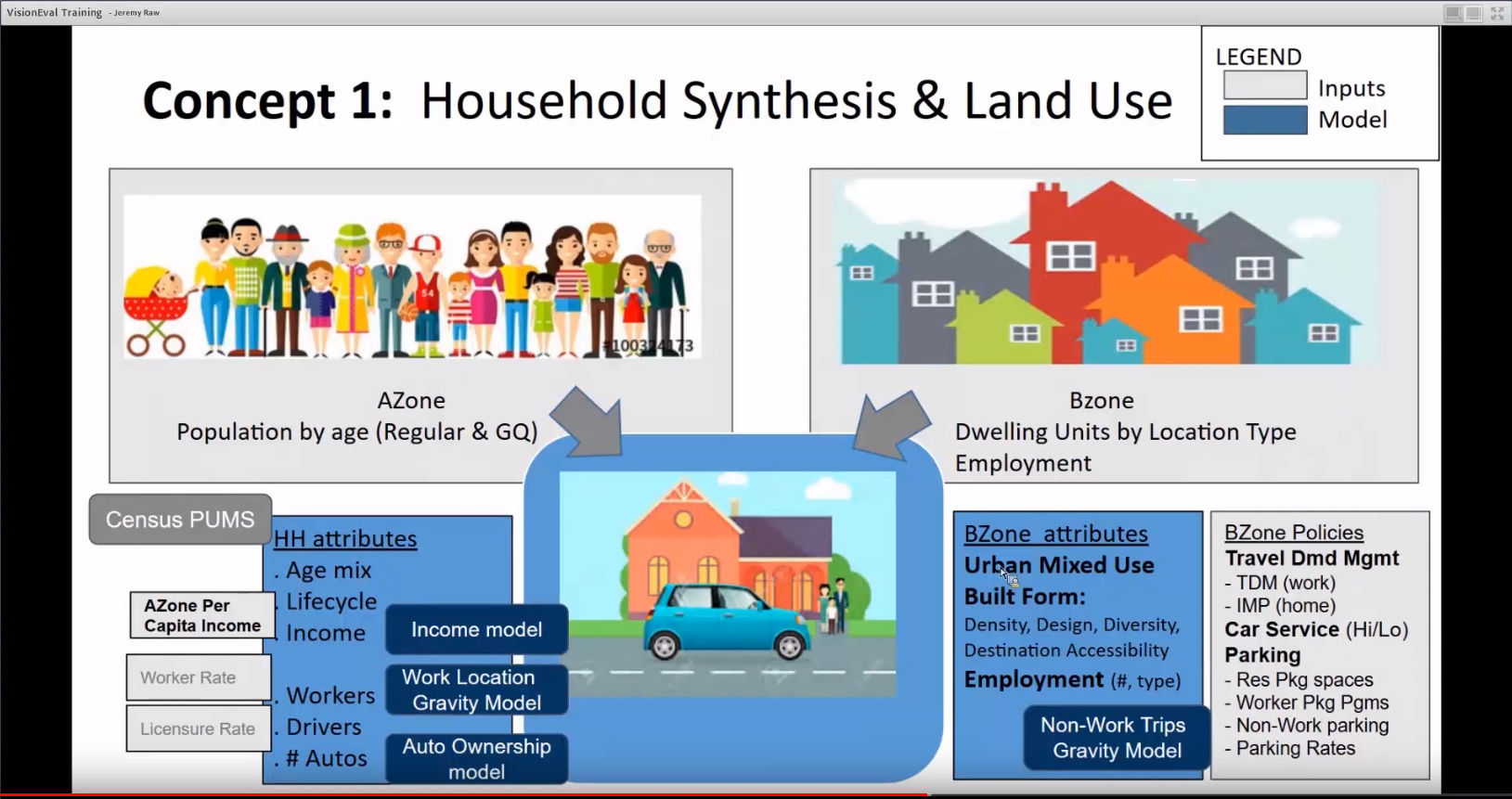
One of the strengths of VisionEval is the rich detail on individual households. This allows for household specific policies, travel behavior can respond to specific household costs and attributes, and outputs can be mined for differences by population groups. The approach of building on a synthesized set of each household borrows from the most recent activity based travel demand models.

VisionEval takes user input statewide population by age group, assembles them into households with demographic attributes (lifecycle, per capita income) and allocates them to BZone-level dwelling units inputs. Separately BZones are attributed with employment and land use attributes (location type, built form ‘D’ values, mixed use, employment by type). Household members are identified as workers and/or drivers and number of household vehicles are estimated. Each home and work location is tied to a specific Bzone with its associated attributes.

Policies are added that apply to each Bzone and thus to households via their assigned home and work location Bzone:

• Parking restrictions (work and nonwork)
• Travel Demand Management programs (home and work-based)
• CarService program availability

The following sections describe each module that contributes to this concept.

Video overview of Household Synthesis and Land Use:

FOR MORE INFORMATION: definitions, inputs, best practices, HouseholdsTutorials, HouseholdsTrainingNotes

Synthesize Households

Customize PUMS Dataset. MUST BE DONE BEFORE RUNNING A MODEL. Prepares a household dataset from Census PUMS for the local area. The default data in the VESimHousehold package is for Oregon. PUMs data for other regions may be used instead, rebuilding the package to reflect Census households for the region of interest.

Create Households. PUMS-identified types of sample households are expanded to meet user control totals and other demographic inputs. Census PUMS (public use micro-sample) data provide probabilities that a person in one of the 6 age groups would be found in each of hundreds of household types.

• Regular households: the module uses a matrix balancing process to allocate persons by age to each of the PUMS household types, in a way that matches input control totals and optional constraints.
• Non-institutional group quarters households are simulated as single-person households.

Predict Workers. The number of workers by age group within each simulated household is predicted using Census PUMS probabilities.

Assign LifeCyle. Categorizes households into 6 lifecycle categories given household age mix and employment status.

Predict Income. The annual income for each simulated household is predicted as a function of the household's worker count by age group, the average per capita income where the household resides(AZone), and interactions between neighborhood income and age (all and seniors) . The models are estimated with Census PUMS data.

Household Drivers and Autos

Assign Drivers. Assigns drivers by age group to each household as a function of the numbers of persons and workers by age group, the household income, land use characteristics, and transit availability. Metropolitan areas are also sensitive to transit service level and urban mixed use home location. Optional restriction on drivers by age group, can be used in calibration or to address trends such as lower millennial licensure rates].

Assign Vehicle Ownership. Determines the number of vehicles owned or leased by each household as a function of household characteristics, land use characteristics, and transportation system characteristics. Households in metropolitan areas are also sensitive to transit service level and urban mixed use home location. First predicts no vehicle households, and then the number of vehicles owned (up to 6), if any.

Land Use Attributes

Calculate 4D Measures. Several land use built form measures by Bzone are calculated: Density, Diversity, & Destination accessibility are calculated based on BZone population, employment, and dwelling unit datasets and developable land area inputs. Design is a user input.

Calculate Urban Mixed Use Measure. An urban mixed-use measure for the household is calculated, based on population density of the home Bzone and dwelling unit type. The model is based on 2001 NHTS data. The model iterates to match an optional input target on the share of households to locate in urban mixed use areas.

Land Use-Household Linkages

Assign Location Types. Households are assigned to land use location types: Urban, Town, Rural. Random assignment based on the household’s dwelling type and input proportions on the mix of dwelling types in each location type of the Bzone.

Predict Housing. Land Use dwelling type[SF, MF,GQ] are assigned to to regular and group quarter households based on the input BZone supply of dwelling units by type. Residential households also consider the relative costliness of housing within the AZone (logged ratio of the household’s income relative to the AZone's mean income), household size, oldest age person, and the interaction of size and income ratio.

Locate Employment. The number of input jobs by Bzone and employment type [retail, service, total] are scaled so that total jobs equals total household workers within the Marea. A worker table is developed and each worker is assigned to a work Bzone. The assignment essentially uses a gravity-type model with tabulations of workers and jobs by Bzone (marginal controls) and distance between residence and employment Bzones (IPF seed, inverse of straight-line distances between home and all work BZone centroids).

Policy Levers

Assign Parking Restrictions. Households are assigned specific parking restrictions and parking fees for their residence, workplace(s), and other places they are likely to visit based on parking inputs by BZone (Metropolitan area only).

• Residential Parking Restrictions & Fees. The number of free parking spaces available at the household's residence is set based on input value that identify the average residential parking spaces by dwelling unit type in each Bzone. For household vehicles that can't be parked in a free space, a residential parking cost (part of auto ownership costs) is identified given input parking rates for the home Bzone if any.

• Employer Parking & Fees. Which workers pay for parking is set by inputs that define the proportion of workers facing parking fees in each Bzone. Whether their payment is part of a cash-out-buy-back program, is similarly set by input proportions by Bzone, and associated fees set by input parking rates for the work Bzone.
• Non-work Parking Fees. The cost of parking for other activities such as shopping is estimated as the likelihood that a household would visit each Bzone and the parking fee in that Bzone. The likelihood is calculated with a gravity-type model, given the relative amount of activity in the Bzone (numbers of households by Bzone and the scaled retail and service job attractions by Bzone as marginals) and the proximity to each destination (inverse distance matrix from home Bzone seed matrix). The average daily parking cost is a weighted average of the fee faced in each destination bzone and the likelihood of visiting that Bzone.

Assign Demand Management. Households are assigned to individualized marketing programs based on input participation levels within their home Bzone. Each worker in the household can also be assigned to an employee commute options program based on input participation levels for workers within their assigned work Bzone. A simple percentage reduction in household VMT is applied based on the household's participation in one or more of these program (maximum of multiple program participation, to avoid double-counting). Worker reductions are only applied to that worker's work travel portion of overall household VMT, and summed if multiple workers in the household participate in such programs.

CAUTION: The model assumes high-caliber TDM programs are in place that produce significant VMT savings. Inputs should reflect this.

Assign CarSvc Availability. Car service level is assigned to each household based on the input car service coverage for where the household resides (Bzone). High Car Service availability can have an impact on auto ownership costs (which affects number of autos owned by the household), and auto operating cost Concept #5.

2. Household Multi-modal Travel

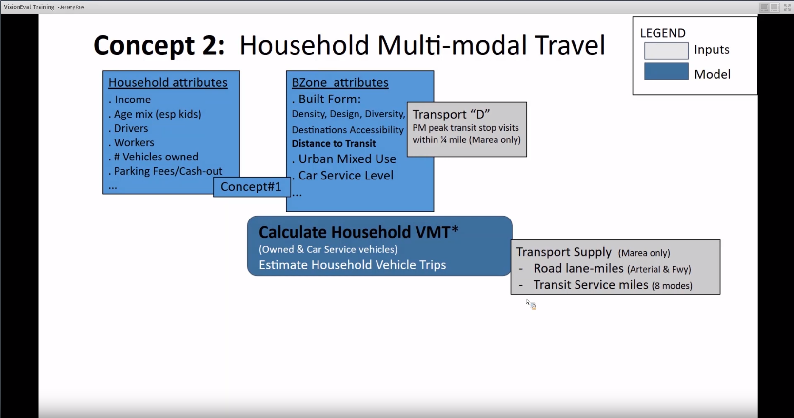
Travel of various modes by households (vehicle, transit, bike, and walk modes) is estimated as a simple function of the rich demographic and land use attributes of the household see Concept #1. In metropolitan areas, travel is also influenced by inputs on transport supply on a per capita basis, i.e., available roadway capacity and bus-equivalent transit service levels. Compared to traditional travel models that build up trip purpose and Origin-Destinations of trips tied to network, VisionEval uses simple regression equations that directly estimate trips and miles by mode (linked by average trip lengths).

After adjusting VMT for household' budget limitations Concept #5, household VMT is further adjusted for household participation in TDM (home & work-based) and short trip SOV diversion, before calculating household trips for all modes. The household's bike miles are also adjusted to reflect SOV diversion input.

The following sections describe each module that contributes to this concept.
The modules are performed in this sequence, including budget adjustments in Concept#5: (1) CalculateHouseholdDvmt with adj (cashout, payd, carSvc) (2) CalculateVehicleOperatingCost (3) Adjust it to fit within BudgetHouseholdDvmt (4) ApplyDvmtReductions due to TDM/IIMP and Short Trips SOV Diversion. (5) 'CalculateVehicleTrips' and 'CalculateAltModeTrips'.

Video overview of multi-modal travel:

FOR MORE INFORMATION: definitions, inputs, best practices, Tutorials,or TrainingNotes

Transport Supply (Metropolitan areas only)

Assign Transit Service. In Metropolitan areas, transit service levels are input. to the metropolitan area and neighborhoods (Bzones). MArea-wide annual revenue-miles (i.e. transit miles in revenue service) by 8 transit service modes are read from inputs. A bzone-level Transit D attribute establishes metropolitan household's access to transit (not yet work access), based on inputs on relative transit accessibility. Using factors derived from the National Transit Database (NTD), input annual transit service miles of each of the 8 transit mode are converted to bus-equivalent-miles by 3 transit vehicle types (van, bus, and rail). Computes the relative transit supply, bus-equivalent service-miles per capita.

Assign Road Miles. Stores input on the numbers of freeway lane-miles and arterial lane-miles by Metropolitan area and year. Computes the relative roadway supply, arterial and freeway lane-miles per capita.

Household Vehicle Travel

Calculate Household Dvmt. Household average daily vehicle miles traveled (VMT) is estimated as a function of household characteristics(income, workers, kids, drivers), vehicle ownership, and attributes of the neighborhood (population density) and metropolitan area (urban mixed-use, transit service level, road lane-miles) where the household resides. It also calculates household VMT percentiles which are used by other modules to calculate whether a household is likely to own an electric vehicle (EV) and to calculate the proportions of plug-in hybrid electric vehicles (PHEV) VMT powered by electricity. First, households with no VMT on the travel day are identified. Then VMT is estimated for those that travel. Average and VMT quantiles are estimated to reflect day-to-day variance that helps identify whether an EV vehicle is feasible for this households typical travel. Uses NHTS2001 dataset.

CalculateVehicleTrips This module calculates average daily vehicle trips for households consistent with the household VMT. Average length of household vehicle trips is estimated as a function of household characteristics (drivers/non-driers, income), vehicle ownership (auto sufficiency), and attributes of the neighborhood (population density) and metropolitan area (urban mixed-use, freeway lane-miles) where the household resides, and interactions among these variables. The average trip length is divided into the average household VMT to get an estimate of average number of daily vehicle trips.

Household Non-vehicle Travel

Calculate AltMode Trips. This module calculates household transit trips, walk trips, and bike trips. The models are sensitive to household VMT so they are run after all household VMT adjustments (e.g. to account for cost on household VMT) are made. Twelve models estimate trips for the 3 modes in metropolitan and non-metropolitan areas, in 2-steps each. The first step determines whether a household has any altmode trips and the second part determines the number of trips. All of the models include terms for household characteristics (size, income, age mix) and the household's overall VMT. Neighborhood factors (population density) factors into all but the bike trip models. For households in metropolitan areas transit service level has an impact as well, with transit ridership also sensitive to when residents live in urban mixed-use neighborhoods.

Household Travel Policy Adjustment

Divert Sov Travel. Household single-occupant vehicle (SOV) travel is reduced to achieve bike and micro-transportation input policy goals, i.e., for diverting a portion of SOV travel within a 20-mile tour distance (round trip distance). This allows evaluating the potential for light-weight vehicles (e.g. bicycles, electric bikes, electric scooters) and infrastructure to support their use, in reducing SOV travel. First, he amount of the household's VMT that occurs in SOV tours having round trip distances of 20 miles or less is estimated. Then the average trip length within those tours is estimated. Both models are sensitive to household characteristics(drivers, income, kids), vehicle ownership (auto sufficiency), and attributes of the neighborhood (population density, dwelling type) and metropolitan area (urban mixed-use, freeway lane-miles) where the household resides, and the household's overall VMT. Both models have multiple stages, including stochastic simulations to capture day-to-day variations.

The diversion of these short trips is assumed to only apply in urban and town location types. The VMT reductions are allocated to households as a function of the household's SOV VMT and (the inverse of) SOV trip length. In other words, it is assumed that households having more qualifying SOV travel and households having shorter SOV trips will be more likely to divert SOV travel to bicycle-like modes. The estimates of the household's share of diverted VMT, average trip length of diverted VMT are applied elsewhere to reduce DMVT and increase bike trips. Zero vehicle households are not allowed to divert SOV travel. Census PUMS data is used to estimate the models.

Apply Dvmt Reductions. Each household's VMT is adjusted for their Travel Demand Management program(s) participation. if any, as well as input from metropolitan-area Short Trips SOV diversion goals. The SOV diversion also increases bike trips (diverted SOV VMT divided by SOV average trip length).

3. Vehicles & Fuels & Emissions

Identifying powertrains and fuels, and associated emissions for all modeled vehicle groups includes some of the most complex datasets used in VisionEval. To simplify for the user, default datasets are included in the downloaded package, having been already processed when the package was built. The user can use these defaults as is, or adjust a constrained set of vehicle, fuel, and emission inputs to represent alternative scenarios. Over time, alternative packages are anticipated to be developed representing different default datasets or policy options. For example, one package may represent a base scenario of federal vehicle, fuel, and emission standards, while another package represents the California zero-emissions vehicle (ZEV) rules and low carbon fue home location's CarService level. Attributes of each vehicle are then estimated. Using estimates of vehicle type and vehicle age the model looks in the correct household vehicle sales table, to determine the probability of each powertrain in that sales year, along with its associated fuel efficiency, etc. Each household vehicle is assigned attributes consistent with these probabilities. Some EVs are replaced by PHEVs if household VMT and residential charging limitations exist.

The powertrain mix of non-household vehicle groups - car service, commercial service, transit, and heavy trucks -- is applied to VMT (rather than individual vehicles) in the scenario year (rather than sales year). There is some input adjustment for average vehicle age and commercial vehicle vehicle type share.

Fuels for each vehicle groups can rely on the package defaults, or use one of two input options. The user can either provide a composite carbon intensity representing all gallons of fuel used for that vehicle group, or provide fuel mix shares (base fuel mix, biofuel blend proportions), combined with package default lifecycle (well-to-wheels) carbon intensity for the individual fuels. The resulting carbon intensity per gallon are applied to gallons generated from VMT and vehicle fuel efficiency assumptions. Concept #4 adjusts fuel efficiency due to reduced speeds from congestion as well as ITS-Operational programs, including [Speed-Smoothing], and EcoDrive programs.

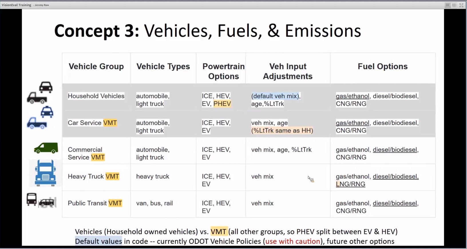
The table below summarizes the vehicle and fuel options available within VisionEval.

Powertrain and Fuels - Available Options by Vehicle Group

Vehicle Group	Vehicle Types	Powertrain Options	Veh Input Adjustments	Fuel Options
Household Vehicles	automobile, light truck	ICE, HEV, EV, PHEV	(default veh mix), age, %LtTrk	gas/ethanol, diesel/biodiesel, CNG/RNG
Car Service VMT	automobile, light truck	ICE, HEV, EV	veh mix, age (HH %LtTrk)	gas/ethanol, diesel/biodiesel, CNG/RNG
Commercial Service VMT	automobile, light truck	ICE, HEV, EV	veh mix, age, %LtTrk	gas/ethanol, diesel/biodiesel, CNG/RNG
Heavy Truck VMT	heavy truck	ICE, HEV, EV	veh mix	gas/ethanol, diesel/biodiesel, CNG/LNG
Public Transit VMT	van, bus, rail	ICE, HEV, EV	veh mix	gas/ethanol, diesel/biodiesel, CNG/RNG

Note: Individual vehicles are modeled for households, based on sales year default datasets and age of the owned vehicle. Other groups' vehicle and fuel attributes apply to VMT in the scenario modeled year. As a result, PHEVs don't exist other than household vehicles, instead PHEVs are represented as miles driven in HEVs and miles in EVs.

The following sections describe each module that contributes to this concept.

Video overview of Vehicles, Fuels, and Emissions

FOR MORE INFORMATION: definitions, inputs, best practices, CongestionTutorials, CongestionTrainingNotes

Household Vehicle Table

Create Vehicle Table. Creates a vehicle table with a record for every vehicle owned by the household, and additional vehicle records are added to reach the household’s number of driving age persons. Each vehicle record is populated with household ID and geography fields (azone, marea) and time-to-access vehicle attributes. Each vehicle record is either “own” or (worker without a vehicle) assigned access to a Car Service level, depending upon coverage in the household’s home Azone.

Assign Vehicle Type. Identifies how many household vehicles are light trucks and how many are automobile as a function of number of vehicles, person-to-vehicle and vehicle-to-driver ratios, number of children, dwelling unit type, income, density, and urban mixed use (in metropolitan areas).

Powertrains And Fuels Defaults.

Load Default Values. RUNS BEFORE MODEL RUN STARTS. This script reads in and processes the default powertrains and fuels files in the package and creates datasets used by other modules to compute fuel consumption, electricity consumption, and via fuel and electricity carbon intensity, emissions from vehicle travel.

Initialize. RUN AUTOMATICALLY BY VISIONEVAL WHEN THE MODEL IS INITIALIZED. Optional user-supplied vehicle and fuel input files, if any, are processed (including input data checks). When available, modules that compute carbon intensities of vehicle travel will use the user-supplied data instead of the package default datasets.

Assign Household Powertrains And Fuels.

Assign Vehicle Age. Assigns vehicle ages to each household vehicle and Car Service vehicle used by the household as a function of the vehicle type (household vehicles only), household income, and assumed mean vehicle age by vehicle type and Azone. The age model starts with an observed (NHTS2001) vehicle age distribution and relationship between vehicle age and income. Adjustments, based on user average vehicle age inputs (household by vehicle type, car service overall).

Assign Household Vehicle Powertrain. This module assigns a powertrain type to each household vehicle. The age of each vehicle is used with default tables by Vehicle Type that identify the powertrain mix of vehicles sold in each sales year. Other default tables identify vehicle characteristics tied to powertrain, including: battery range, fuel efficiency, and emissions rate . Assignments of EVs may be changed to PHEVs if the battery range is not compatible with estimated day-to-day trip lengths, or the home dwelling lacks vehicle charging availability.

Calculate Carbon Intensity. This module calculates the average carbon intensity of fuels (grams CO2e per megajoule) by vehicle group and if applicable, vehicle type. Average fuel carbon intensities for transit vehicle modes are calculated by Metropolitan area, other vehicles are calculated for the entire model region. The module also reads the input average carbon intensity of electricity at the Azone level.

Assign Non-Household Powertrains And Fuels.

Calculate Transit Energy And Emissions. This module calculates the energy consumption and carbon emissions from transit vehicles in urbanized areas. Assumptions (package default or user input) onpowertrain mix and fuels for three transit vehicle types by Metropolitan area, are applied to associated Metropolitan area transit service miles for these types [Concept#3]. Assumptions (package default or user input) on average carbon intensity of fuel and electricity by transit vehicle types are then applied to Metropolitan area fuel and electricity usage across types to calculate carbon emissions.

Calculate Commercial Energy And Emissions. The energy consumption and carbon emissions of heavy trucks and commercial service VMT (no vehicles) are calculated by on-road (not sales) year. VMT shares of Commercial Service powertrains by vehicle type and Heavy truck powertrains are calculated (package default or user input). Any fuel efficiency (MPG and MPKWH) adjustments are then applied, due to policies (ecodriving, ITS speed-smoothing) and/or congestion (including effects of any ITS-operational and congestion fee policies)see Concept #4. Ecodriving applies only to ICE vehicles, and ITS-operational policies and congestion apply only in Metropolitan area. Both vary by powertrain and for commercial vehicles, vehicle type. Combining fuel efficiency and VMT Concept #2 results in estimates of energy usage (fuel and electricity). Fuel carbon intensity for these modes is calculated by Metropolitan area and/or region and applied to fuel and electricity usage to estimate CO2e emissions.

4. Congestion Adjustment

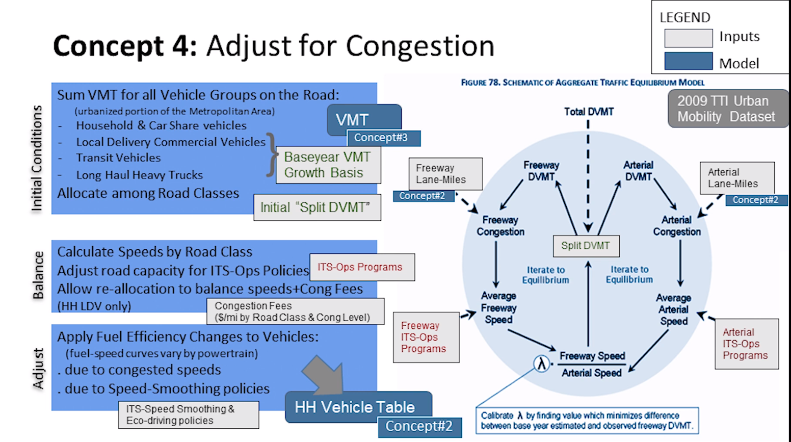
Congestion, only calculated on urbanized roads, a subset of metropolitan area roads, requires estimating and combining together the VMT of all Vehicle Groups. For non-household vehicles, baseyear VMT is calculated directly from inputs and model parameters, while future year is a function of the input growth basis. Initial allocations of DMVT across road class is based on input values.

LDV VMT is allowed to re-allocate between freeways and arterials to balance demand (VMT) and roadway supply (lane-miles) through a generalized cost framework (including roadway speed and congestion fees, if any). Roadway supply (i.e., capacity) is adjusted by delay-reducing ITS-operations policies. Based on fuel-speed curves by powertrain, the resulting congested speeds impact vehicle fuel-efficiency. Further adjustments are applied to reflect any ITS-speed smoothing and eco-drive programs that may not affect delay but reduce acceleration and deceleration with associated impacts on fuel efficiency. xxxNo fuel efficiency adjustments for congestion or policies are made to non-urban roadway VMT. The delays faced by each household and associated fuel economy impacts are applied to each individual household's VMT and vehicles. Resulting overall average speeds, delays, and DMVT proportions, by road class at each congestion level on urbanized and other roads are also tabulated along with the resulting average per mile congestion fees paid, if any, and overall [vehicle hours of delay (VHD)] by vehicle group.

Video overview of congestion adjustment:

FOR MORE INFORMATION: definitions, inputs, best practices, Tutorials,TrainingNotes

Initialize Roadway Conditions

Load Default Road VMT Values. RUNS BEFORE MODEL RUN STARTS. Baseyear roadway VMT is processed. This includes LDV & Heavy Truck VMT by state and urbanized area as well as VMT proportions by urbanized area, vehicle group(LDV, Heavy truck, bus), and road class (freeway, arterial, other). The user can either provide direct inputs for these values or specify a state and/or urbanized area and the model will use default data from the 20xxx USDOT Highway Statistics, where available.

Initialize. RUN AUTOMATICALLY BY VISIONEVAL WHEN THE MODEL IS INITIALIZED. User inputs used by several modules are read and checked (many with several valid options, proportions sum to 1, consistency, congestion fees increase with congestion level). Some of these values are optional, using default data where not specified. This includes various assumptions on baseyear VMT within both urbanized area and the full model region, by vehicle group; allocation among road class; growth basis assumptions for freight vehicle groups. It also checks inputs on ITS-operational policies and eco-driving programs, including any user-specified 'other ops' programs, and congestion fees (by road class and congestion level)

Calculate Road VMT. Adds together metropolitan area VMT of all vehicle groups (Households, CarService, Commercial Service, Heavy Truck, Transit) and allocates it across road class(freeway, arterial, other) limiting it to urbanized area roadways for use in congestion calculations. To do so, several factors are established in the baseyear. One uses the input growth basis (population, income, household VMT) to estimate future year freight vehicle group (Commercial service and heavy truck) VMT (using input baseyear VMT values by region and marea, if provided, model-estimates otherwise). A second baseyear factor identifies the urban and non-urban allocation of VMT from metropolitan area households and related commercial service vehicles. For Heavy Trucks VMT, an input specifies the proportion of VMT on urbanized roads while transit VMT (of all Transit service modes) is assumed to only occur on urbanized roads. Baseyear allocations of urban VMT by vehicle group among road classes are based on input shares, subject to adjustment during subsequent congestion calculations. Finally, to assess delay faced by each household and associated fuel efficiency impacts, each individual household's VMT is split between miles on urbanized and other road miles.

Congestion Model & Adjustments

Calculate Road Performance. Congestion level by road class and the associated amounts of VMT are iteratively estimated. LDV VMT is allowed to re-allocate between freeways and arterials to balance demand and roadway supply (lane-miles) through a generalized cost framework (including roadway speed and congestion fees, if any and an estimated baseyear urbanized area lambda parameter based on the area's population and freeway-arterial lane-mile ratio). DMVT allocation at different aggregate demand-supply ratios relies on data from the 2009 Urban Mobility Study (UMS) for 90 urbanized areas, where the model chooses the 5-10 cities with most similiar congestion ratios.

The supply calculation considers the delay-reduction effects of deploying urban area ITS-operations programs (freeway ramp metering, freeway incident management, arterial signal coordination, arterial access control or user-defined 'other ops' programs. The standard ITS-operations program impacts are based on research (Bigazzi and Clifton, Task 2 Report, 2011). Non-urban speeds are also calculated, using a simple ratio of rural-to-urban travel volumes.

The resulting average speeds, delay and DMVT proportions, by road class at each congestion level on urbanized and other Metropolitan area roads are calculated; as is the resulting average per mile congestion fees paid, if any, and overall [VHD] by vehicle group.

Calculate Mpg Mpkwh Adjustments. Adjustments to fuel efficiency (MPG and MPKwhr) for all Vehicle Groups resulting from traffic congestion, congestion fees, ITS-speed smoothing (i.e. active traffic management which reduces speed variation), and eco-driving are calculated. The fuel-speed curves vary by road class, congestion powertrains (LdIce, LdHev, LdEv, HdIce) and, where applicable vehicle type, relative to reference speeds by road class. The adjustments are based on drive-cycle level simulation research (Bigazzi and Clifton, Task 1 Report, 2011).

Note: No adjustments are made for ITS policies (standard and speed smoothing policies) or eco-drive programs on 'other' road classes (non-freeway or arterials) and non-urbanized roads, which are assumed to be uncongested.

Adjust Household Vehicle MPg Mpkwh. Implements the fuel efficiency (MPG and MPKwh) adjustments of household vehicles (including Car Service VMT), reflecting the effects of congestion, congestion fees, ITS-speed smoothing, and eco-driving that were calculated elsewhere. These adjustments vary by vehicle powertrain, vehicle type, and the proportion of the household's travel that is driven on urban and non-urban[xxxsame as rural?] roads within the metropolitan area. Joint effects are calculated as the product of congestion speed effects and the maximum of implemented speed-smoothing policies (eco-driving & ITS-speed smoothing).

5. Household Costs & Budgets Adjustment

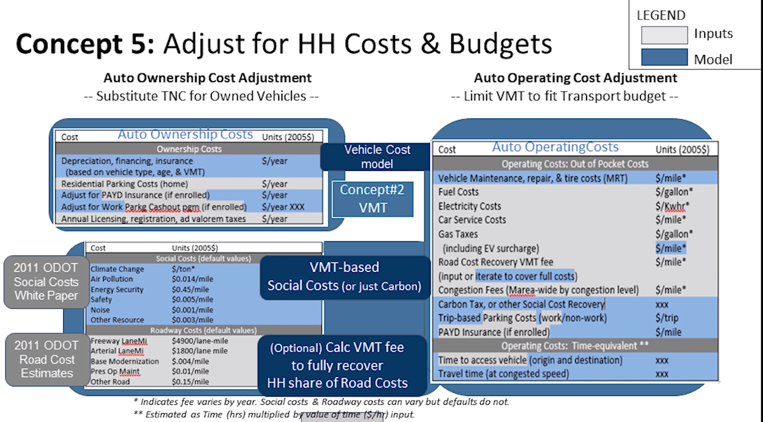
Two adjustments are made in response to household budgets. Auto ownership costs are calculated and an adjustment is made to the number of household owned autos if the costs are less than switching to a 'High' level Car Service, where available (subject to input limits on Car Service substitutability). Vehicle ownership costs include financing, depreciation, insurance (unless in PAYD program), annual registration fees, and residential parking fees.

Additionally, in order to respond to pricing policies and energy costs, VisionEval imposes a budget limitation. Household VMT is constrained such that annual vehicle operating costs must stay below a maximum share of annual household income, or budget limit. A household-specific average annual vehicle operating costs is first calculated, including out-of-pocket per mile costs for each household owned and Car Service vehicles used by the household, as well as time-equivalent cost (input access times, estimates of VMT at congested speeds, and value-of-time input). Vehicle operating costs determine the proportional split of VMT among household vehicles. Out-of-pocket costs include the energy, [Maintenance, Repair, & Tires], road use taxes (including EV surcharge and optional calculation of fee to fully recover road costs), work/non-work parking, PAYD insurance, input share of carbon and other social costs, as well as CarService fees by the household.

The following sections describe each module that contributes to this concept.

Video overview of costs and budgets:

FOR MORE INFORMATION: definitions, inputs, best practices, Tutorials,or TrainingNotes

Auto Ownership Cost & Adjustment

Calculate Vehicle Own Cost. Average vehicle ownership costs are calculated for each vehicle based on the [vehicle type], age, and annual VMT (financing, depreciation, and insurance), annual registration fees (flat and ad valorum), combined with any residential parking fees (if household exceeds free parking limits). To do so, PAYD insurance participation is assigned based on household characteristics (drivers by age, annual mileage, income, location type, vehicle type and age) and input PAYD insurance program participation. The ownership cost is converted into an average vehicle-specific ownership cost per mile by dividing by estimated household VMT per vehicle.

NOTE: PAYD insurance does not affect the cost of vehicle ownership when determining whether a household will substitute car services for one or more of their vehicles. It does affect the out-of-pocket operating cost used in budget limitations on household VMT.

Adjust Vehicle Ownership. Household vehicle ownership is adjusted based on a comparison of the cost of owning versus 'high' car service per mile ratesConcept #2, where available. The module identifies all household vehicles in a 'High' car service area, where the car service mileage rate exceeds the household's estimated vehicle ownership cost per annual household VMT. The Household's vehicle table entry changes from 'Own' to 'HighCarSvc' for these vehicles, limited by input assumptions regarding the average likelihood that an owner would substitute car services for a household vehicle (separate values are specified by Vehicle Type). Other auto ownership values are also updated (insurance, total vehicles, etc.).

Auto Operating Cost & Adjustment

Calculate Vehicle Operating Cost. A composite per mile cost is calculated as an out-of-pocket cost for various household and Car Service vehicle VMT (see below), combined with cost equivalent of travel time (access time and travel time at congested speeds times Value-of-time (VOT)`). Total costs result from applying this vehicle-specific cost rate to each vehicle's VMT, where VMT is split among household vehicles (including car services used by household members) as a (reciprocal) function of this vehicle-specific composite cost rate:

• Vehicle maintenance, repair, and tire cost (MRT). Calculated as a function of the vehicle type, powertrain and vehicle age based on data from the American Automobile Association (AAA) and the Bureau of Labor Statistics (BLS).
• Fuel and energy costs. Calculated as energy rates time average fuel efficiency (miles per gallon or Kwhr electricity).
• Gas taxes. Federal, state and local per gallon taxes to cover road costs. For Electric vehicles, an equivalent per mile cost is calculated and can be applied to some or all electric vehicles ($/gallon or EV vehicle surcharge tax).
• Other Road Cost Recovery taxes (i.e. VMT tax) is a user input. If the (optional) BalanceRoadCostsAndRevenues module is run, an extra VMT tax is calculated that recovers household share of road costs, consistent across all model households.
• Congestion fees. Calcluated average congestion price ($/mile) for travel on urbanized roads in the Marea multiplied by the proportion of household travel occurring on those roads.
• Carbon fee & other social cost fees: Carbon cost per mile is calculated as the input price of carbon times the average household emissions rate (grams/mile), a VMT-weighting of all vehicles in the household. Of the other social costs, some are per gallon (non-EV vehicle miles) others per mile (regardless of powertrain). The full per mile costs are discounted to only reflect the input proportion of social cost paid by user.
• Parking costs: Daily parking costs from work parking costs (workers who pay for parking) and other parking cost (cost of parking for shopping, etc.) are summed and divided by the household DMVT. NOTE: Residential parking costs are included in the vehicle ownership not per mile cost calculations.
• Pay-as-you-drive (PAYD) insurance: For participating households the sum of the annual insurance cost for all the household vehicles is divided by the annual household VMT.
• Car-service costs: The cost of using a car service (dollars/mile) is a user input by car service level (Low, High).

Balance Road Costs And Revenues. Optionally, an extra mileage tax ($/mile) for household vehicles needed to make up any difference in the cost of constructing, maintaining, and operating roadways and the revenues from total road cost fees including fuel, VMT, and congestion charges. Optionally, an additional mileage fee ($/mile) on household travel is calculated that would fully pay for roadway costs attributable to household vehicle travel. The cost of existing and new freeway and arterial lane-miles by Marea is calculated from the difference in input lane-miles relative to the base year and input unit road costs (constructing, maintaining, and operating). Reductions in lane-miles are ignored. The proportion of road costs attributable to households is set as the ratio of household VMT divided by the sum of household (including CarService), commercial service, and car-equivalent heavy truck VMT (multiply by PCE). Average road taxes collected per household vehicle mile are calculated as a weighted average of the average road tax per mile of each household (calculated by the 'CalculateVehicleOperatingCost' module) using the household VMT (calculated by the 'BudgetHouseholdDvmt' module) as the weight. Currently no annual fees contribute to road cost recovery.

Budget Household Dvmt. Household VMT is adjusted to keep within the household's vehicle operating cost budget, based on the historic maximum proportion of income the household is willing to pay for vehicle operations. This proportions varies with income. The household's DMVT is then reduced as needed to keep annual vehicle operating cost within that share of the household's annual income. Annual vehicle operating costs include the household's VMT times their own per mile vehicle costs, adding credits for selected annual payments (annual work parking fee if in a work parking cash-out-buy-back program, annual vehicle insurance if in a PAYD insurance program, and annual auto ownership costs if car service program reduced auto ownership). The module relies on aggregate survey data from the U.S. Bureau of Labor Statistics (BLS) Consumer Expenditure Survey (CES) for years 2003-2015.

Processing & Validation

VisionEval generates a large set of performance metrics at varying summary levels. Several pre-defined metrics are compiled for mobility, economic, land use, environmental, and energy categories in each model run. They can be tabulated for individual scenarios or compared to other scenarios, as well as visualized using VEGUI.

The intermediate data generated during the various VisionEval module steps can be compiled as performance metrics, both in absolute and per-capita terms and at various geographies. Traditional transportation network metrics such as VMT, vehicle and person hours of travel, and total delay are easily compiled by overall or focused areas within the model. Likewise, emission estimates and fuel consumption are tabulated. These can be viewed in standard reports, but often more effectively view in the VEGUI dashboard, especially when comparing such values between scenarios.

One Example of a set of region-wide performance metrics used by Oregon DOT follows:

• Mobility
  • Daily VMT per capita
  • Annual walk trips per capita
  • Daily Bike trips per capita
• Economy
  • Annual all vehicle delay per capita (hours)
  • Daily household parking costs
  • Annual HH vehicle operating cost (fuel, taxes, parking)
  • Annual HH ownerhsip costs (depreciation, vehicle maintenance, tires, finance charge, insurance, registration)
• Land Use
  • Residents liming in mixed use areas
  • Housing type (SF: MF)
• Environmental
  • Annual GHG emissions per capita
  • HH vehicle GHG/mile
  • Commercial vehicle GHG/mile
  • Transit Vehicle GHG/mile
• Energy
  • Annual all vehicle fuel consuption per capita (gallons)
  • Average all vehicle fuel efficiency (net miles per gallon)
  • Annual external social costs per households (total/% paid)

• EXPORTING DATA

Most of the data generated during a VisionEval model run can be exported (using exporter.R) if desired for further analyses. The user can then mine and visualize the data using a variety of open source and proprietary tools. This provides the user with considerable flexibility for creating more detailed statistics than those provided by the program. These VisionEval outputs might further serve as inputs to other models (e.g., emissions models, economic impact models) and visualization tools, and compilation of additional performance metrics.

9. Validation

Setting up the model includes the steps required to apply the model for a given study. It is somewhat related to validation, both for informing what types of studies that VisionEval are appropriately sensitive to and interpreting the results. See the Getting Started page on the wiki for an overview of getting started initially.

There are several options for making adjustments in order to calibrate and validate the models. These adjustments vary in difficulty, and the most appropriate approach varies by module. From easiest to most difficult the options for making adjustments are:

• Self-calibration: Several of the modules are self-calibrating in that they automatically adjust calculations to match input values without intervention by the user.[Selected value should be validated to confirm the calculations are done correctly]
• Adjustment of model inputs: Some modules allow the user to optionally enter data that can be used to adjust the models to improve their match to observed conditions.
• Model estimation data: Several modules use data specific to the region where the model is deployed, such as household synthesis. Functions within each module generate cross-tabulations required from these data. Census PUMS data from Oregon were used to develop the original models, and should be replaced with Census PUMS data for the modeled area.
• Model estimation scripts: An advanced user or developer can make adjustments to the model code itself in order to facilitate better matching observed local behavior or patterns. This, of course, is the most difficult option and opens up potential for significant errors, but it is possible for users that know what they are doing.

The main validation targets have historically included household income, vehicle ownership, vehicle miles of travel, and fuel consumption. The number of workers and drivers within each geography have recently become more widely used. These statistical comparisons can be made for the modeled area as a whole or for large geographies nested within them (e.g., Azones, Mareas). Sensitivity tests should be performed to evaluate the reasonableness (eg. correct direction and magnitude) of the VisionEval output estimates. Comparable community applications of VisionEval may also provide a reasonableness check that the model is functioning appropriately.

Note: HPMS definition of VMT differs from that of VisionEval. VisionEVal reports on all household travel regardless of where it occurs, and adds Commercial vehicle and Heavy Duty Truck and Bus travel on MPO roads. HPMS reports vehicular travel of all modes on roads within the MPO boundary.

Additional detail on model validation can be found here.