Trinity Differential Expression
Our current system for identifying differentially expressed transcripts relies on using the EdgeR Bioconductor package. We have a protocol and scripts described below for identifying differentially expressed transcripts and clustering transcripts according to expression profiles. This process is somewhat interactive, and described are automated approaches as well as manual approaches to refining gene clusters and examining their corresponding expression patterns.
We recommend generating a single Trinity assembly based on combining all reads across all samples as inputs. Then, reads are separately aligned back to the single Trinity assembly for downstream analyses of differential expression, according to our abundance estimation protocol. If you decide to assemble each sample separately, then you'll likely have difficulty comparing the results across the different samples due to differences in assembled transcript lengths and contiguity.
Before attempting to analyze differential expression, you should have already estimated transcript abundance and generated an RNA-Seq counts matrix containing RNA-Seq fragment counts for each of your transcripts (or genes) across each biological replicate for each sample (experiment, condition, tissue, etc.).
If you have biological replicates, be sure to align each replicate set of reads and estimate abundance values for the sample independently, and targeting the single same targeted Trinity assembly.
Trinity provides support for several differential expression analysis tools, currently including the following R packages:
- edgeR : http://bioconductor.org/packages/release/bioc/html/edgeR.html
- DESeq2: http://bioconductor.org/packages/release/bioc/html/DESeq2.html
- limma/voom: http://bioconductor.org/packages/release/bioc/html/limma.html
- ROTS: http://www.btk.fi/research/research-groups/elo/software/rots/
Be sure to have R installed in addition to the above software package that you want to use for DE detection.
In addition, you'll need the following R packages installed: ctc, Biobase, gplots, and ape. These can be installed like so (along with the subset of Bioconductor packages for DE software above)
 % R
 > source("http://bioconductor.org/biocLite.R")
 > biocLite('edgeR')
 > biocLite('limma')
 > biocLite('DESeq2')
 > biocLite('ctc')
 > biocLite('Biobase')
 > install.packages('gplots')
 > install.packages('ape')
If you have R version 3.5 or greater use the commands below to get above packages:
 % R
 > BiocManager::install(c("edgeR", "limma", "DESeq2", "ctc", "Biobase", "gplots", "ape", "argparse"))
Differentially expressed transcripts or genes are identified by running the script below, which will perform pairwise comparisons among each of your sample types. If you have biological replicates for each sample, you should indicate this as well (described further below). To analyze transcripts, use the 'transcripts.counts.matrix' (or isoform.counts.matrix in later software versions) file. To perform an analysis at the 'gene' level, use the 'genes.counts.matrix'. Again, Trinity Components are used as a proxy for 'gene' level studies.
$TRINITY_HOME/Analysis/DifferentialExpression/run_DE_analysis.pl
#################################################################################################
#
#  Required:
#
#  --matrix|m <string>               matrix of raw read counts (not normalized!)
#
#  --method <string>               edgeR|DESeq2|voom
#                                     note: you should have biological replicates.
#                                           edgeR will support having no bio replicates with
#                                           a fixed dispersion setting.
#
#  Optional:
#
#  --samples_file|s <string>         tab-delimited text file indicating biological replicate relationships.
#                                   ex.
#                                        cond_A    cond_A_rep1
#                                        cond_A    cond_A_rep2
#                                        cond_B    cond_B_rep1
#                                        cond_B    cond_B_rep2
#
#
#  General options:
#
#  --min_reps_min_cpm  <string>    default: $MIN_REPS_MIN_CPM  (format: 'min_reps,min_cpm')
#                                  At least min count of replicates must have cpm values > min cpm value.
#                                     (ie. filtMatrix = matrix[rowSums(cpm(matrix)> min_cpm) >= min_reps, ]  adapted from edgeR manual)
#                                      Note, ** if no --samples_file, default for min_reps is set = 1 **
#
#  --output|o                      name of directory to place outputs (default: \$method.\$pid.dir)
#
#  --reference_sample <string>     name of a sample to which all other samples should be compared.
#                                   (default is doing all pairwise-comparisons among samples)
#
#  --contrasts <string>            file (tab-delimited) containing the pairs of sample comparisons to perform.
#                                  ex.
#                                       cond_A    cond_B
#                                       cond_Y    cond_Z
#
#
###############################################################################################
#
#  ## EdgeR-related parameters
#  ## (no biological replicates)
#
#  --dispersion <float>            edgeR dispersion value (Read edgeR manual to guide your value choice)
#                                    http://www.bioconductor.org/packages/release/bioc/html/edgeR.html
#
###############################################################################################
#
#   Documentation and manuals for various DE methods.  Please read for more advanced and more
#   fine-tuned DE analysis than provided by this helper script.
#
#  edgeR:       http://www.bioconductor.org/packages/release/bioc/html/edgeR.html
#  DESeq2:      http://bioconductor.org/packages/release/bioc/html/DESeq2.html
#  voom/limma:  http://bioconductor.org/packages/release/bioc/html/limma.html
#
###############################################################################################
Note, be sure your counts matrix filename ends with '.matrix', so it'll be compatible with the downstream analysis script 'analyze_diff_expr.pl' described below.
It's very important to have biological replicates to power DE detection and reduce false positive predictions. If you do not have biological replicates, edgeR will allow you to perform DE analysis if you manually set the --dispersion parameter. Values for the dispersion parameter must be chosen carefully, and you might begin by exploring values between 0.1 and 0.4. Please visit the edgeR manual for further guidance on this matter.
  $TRINITY_HOME/Analysis/DifferentialExpression/run_DE_analysis.pl \
      --matrix counts.matrix --method edgeR --dispersion 0.1
Be sure to have a tab-delimited 'samples_described.txt' file that describes the relationship between samples and replicates. For example:
conditionA   condA-rep1
conditionA   condA-rep2

conditionB   condB-rep1
conditionB   condB-rep2

conditionC   condC-rep1
conditionC   condC-rep2
where condA-rep1, condA-rep2, condB-rep1, etc..., are all column names in the 'counts.matrix' generated earlier (see top of page). Your sample names that group the replicates are user-defined here.
Note, this can be the same samples.txt file used with Trinity assembly, containing the extra column(s) with paths to the fastq files. The file paths aren't essential here, though.
Any of the available methods support analyses containing biological replicates. Here, for example, here we choose DESeq2 .
  $TRINITY_HOME/Analysis/DifferentialExpression/run_DE_analysis.pl \
          --matrix counts.matrix \
          --method DESeq2 \
          --samples_file samples_described.txt
By default, each pairwise sample comparison will be performed. If you want to restrict the pairwise comparisons, provide the list of the comparisons to perform to the --contrasts parameter (see usage info above).
A full example of the edgeR pipeline involving combining reads from multiple samples, assembling them using Trinity, separately aligning reads back to the trintiy assemblies, abundance estimation using RSEM, and differential expression analysis using edgeR is provided at: $TRINITY_HOME/sample_data/test_full_edgeR_pipeline
The output from running the DE analysis will reside in the output directory you specified, and if not, a default directory name that includes the name of the method used (ie. edgeR/ or DESeq2/).
In this output directory, you'll find the following files for each of the pairwise comparisons performed:
${prefix}.sampleA_vs_sampleB.${method}.DE_results : the DE analysis results,\
including log fold change and statistical significance (see FDR column).
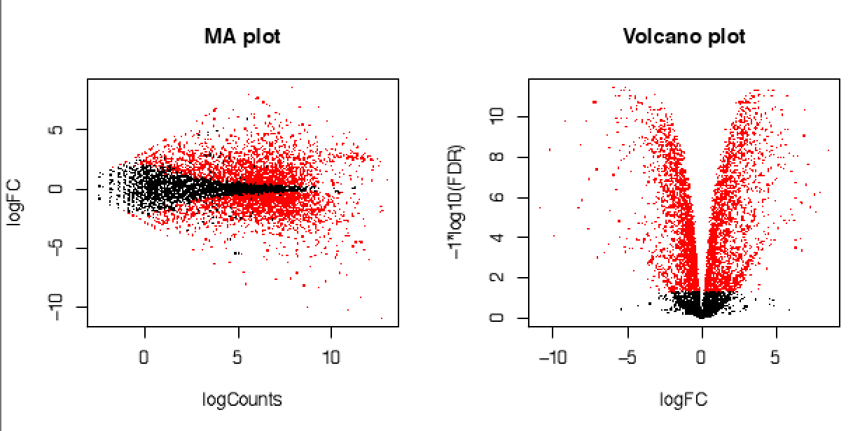
${prefix}.sampleA_vs_sampleB.${method}.MA_n_Volcano.pdf : MA and Volcano plots \
features found DE at FDR <0.05 will be colored red. Plots are shown\
with large (top) or small (bottom) points only for choice of aesthetics.
${prefix}.sampleA_vs_sampleB.${method}.Rscript : the R-script executed to perform the DE analysis.
A top few lines from an example DE_results file is as follows:
| logFC | logCPM | PValue | FDR |
|---|---|---|---|
| TR3679_c0_g1_i1 | -5.11541024334567 | 11.7653852968686 | 7.23188081710377e-16 |
| TR2820_c0_g1_i1 | -5.94194741644588 | 12.0478207481011 | 1.02760683781471e-15 |
| TR3880_c0_g1_i1 | -4.841676068963 | 11.1650356947446 | 2.03198563430982e-15 |
| TR4554_c0_g1_i1 | 3.58688559685832 | 11.4005717047623 | 3.41037012439576e-15 |
| TR2827_c0_g1_i1 | 3.76108564650662 | 11.1790325703142 | 5.01055012548484e-15 |
| TR3686_c0_g1_i1 | 2.9858493815106 | 11.4428280579112 | 6.26951899823494e-14 |
| TR4205_c0_g1_i1 | -4.87460353182789 | 9.68033063079378 | 4.88840211796863e-14 |
| TR574_c1_g1_i1 | 3.79320160636904 | 9.08537961019643 | 8.28450341444472e-14 |
| TR2795_c0_g2_i1 | 2.61077027548215 | 11.0533004315067 | 9.88108242818427e-14 |
| TR734_c0_g1_i1 | 2.75732519093165 | 11.0993615161482 | 1.09213602844387e-13 |
| TR2376_c0_g1_i1 | 2.98740515629102 | 11.0250977284312 | 1.11753237030591e-13 |
| TR4597_c0_g1_i1 | 2.4818510017606 | 11.7495033269948 | 1.11423379517395e-13 |
| ............. | ............. | ............. | ........... |
An example MA and volcano plot as generated by the above is shown below:
The Glimma software provides interactive plots. Generate volcano and MA-plots for any of your pairwise DE analysis results like so:
%  ${TRINITY_HOME}/Analysis/DifferentialExpression/Glimma.Trinity.Rscript \
       --samples_file samples.txt \
       --DE_results file.DE_results \
       --counts_matrix file.counts.matrix
Example interactive Glimma plots are available as: Glimma MA-plot and Glimma volcano plot.
An initial step in analyzing differential expression is to extract those transcripts that are most differentially expressed (most significant FDR and fold-changes) and to cluster the transcripts according to their patterns of differential expression across the samples. To do this, you can run the following from within the DE output directory, by running the following script:
  $TRINITY_HOME/Analysis/DifferentialExpression/analyze_diff_expr.pl


 ###########################################################################################################
 #
 # Required:
 #
 #  --matrix <string>       TMM.EXPR.matrix
 #
 # Optional:
 #
 #  -P <float>             p-value cutoff for FDR  (default: 0.001)
 #
 #  -C <float>             min abs(log2(a/b)) fold change (default: 2  (meaning 2^(2) or 4-fold).
 #
 #  --output <float>       prefix for output file (default: "diffExpr.P${Pvalue}_C${C})
 #
 #
 #
 #
 # Misc:
 #
 #  --samples <string>                     sample-to-replicate mappings (provided to run_DE_analysis.pl)
 #
 #  --max_DE_genes_per_comparison <int>    extract only up to the top number of DE features within each pairwise comparison.
 #                                         This is useful when you have massive numbers of DE features but still want to make
 #                                         useful heatmaps and other plots with more manageable numbers of data points.
 #
 #  --order_columns_by_samples_file        instead of clustering samples or replicates hierarchically based on gene expression patterns,
 #                                         order columns according to order in the --samples file.
 #
 #  --max_genes_clust <int>                default: 10000  (if more than that, heatmaps are not generated, since too time consuming)
 #
 #  --examine_GO_enrichment                run GO enrichment analysis
 #       --GO_annots <string>              GO annotations file
 #       --gene_lengths <string>           lengths of genes file
 #
 #
 ##############################################################################################################
For example, running the following:
 cd voom_outdir/

 $TRINITY_HOME/Analysis/DifferentialExpression/analyze_diff_expr.pl --matrix ../Trinity_trans.TMM.EXPR.matrix -P 1e-3 -C 2
which will extract all genes that have P-values at most 1e-3 and are at least 2^2 fold differentially expressed. For each of the earlier pairwise DE comparisons, this step will generate the following files:
 ${prefix}.sampleA_vs_sampleB.voom.DE_results.P0.001_C2.sampleA-UP.subset : the expression matrix subset \
                                                                        for features up-regulated in sampleA
 ${prefix}.sampleA_vs_sampleB.voom.DE_results.P0.001_C2.sampleB-UP.subset : the expression matrix subset \
                                                                        for features up-regulated in sampleB
and then the following summary files are generated:
diffExpr.P0.001_C2.matrix.log2.dat : All features found DE in any of these pairwise comparisons\
consolidated into a single expression matrix:
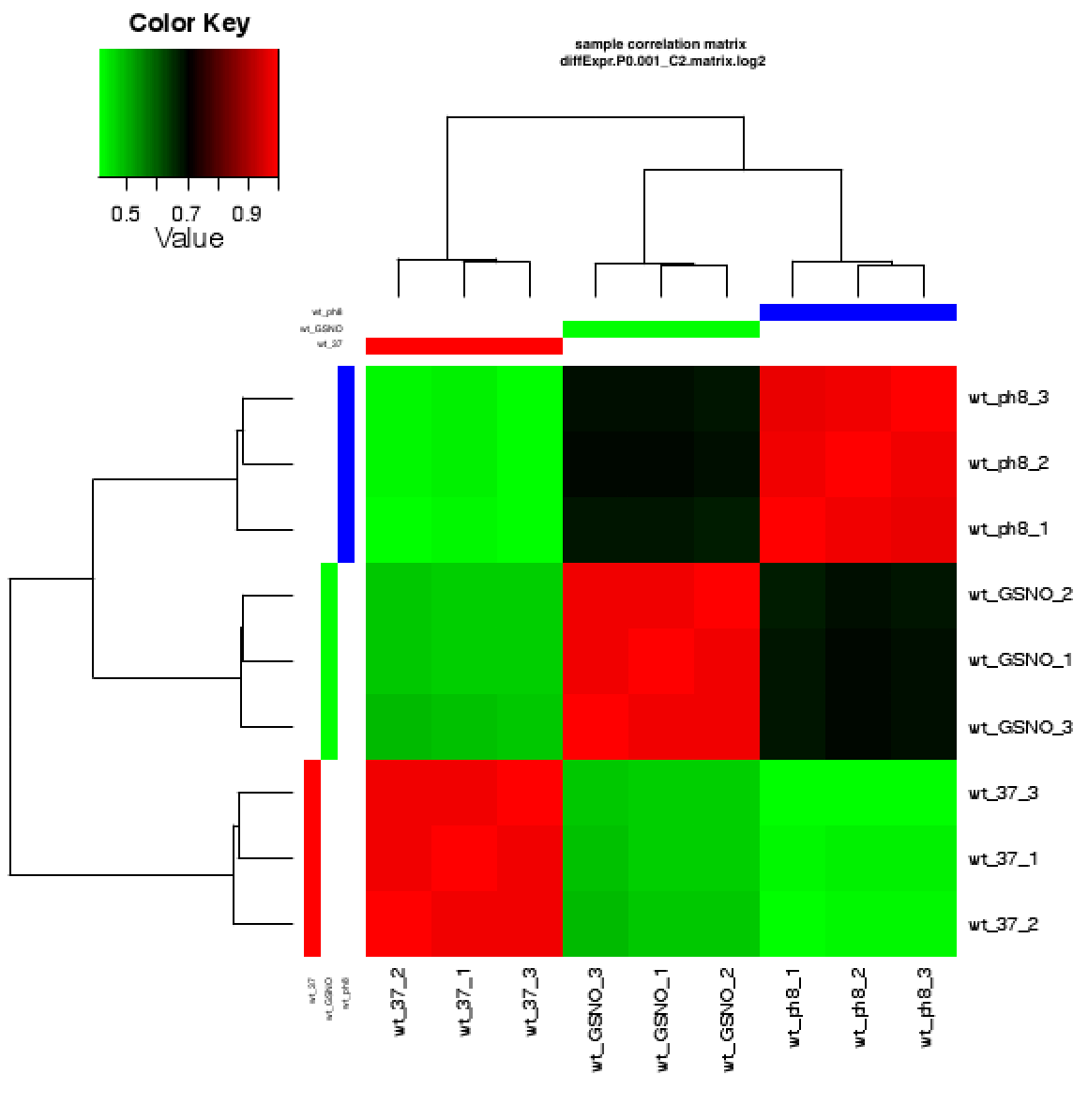
diffExpr.P0.001_C2.matrix.log2.sample_cor.dat : A Pearson correlation matrix for pairwise sample comparisons \
based on this set of DE features.
diffExpr.P0.001_C2.matrix.log2.sample_cor_matrix.pdf : clustered heatmap showing the above sample correlation matrix.
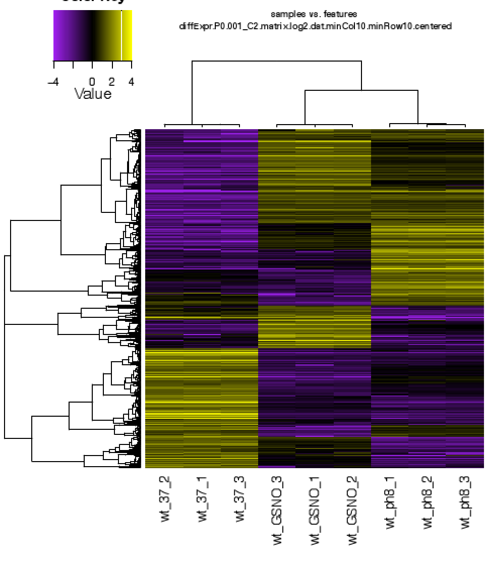
diffExpr.P0.001_C2.matrix.log2.centered.genes_vs_samples_heatmap.pdf : clustered heatmap of DE genes vs. sample replicates.
An example sample correlation matrix heatmap is as follows:
And an example DE gene vs. samples heatmap is as follows:
The above is mostly just a visual reference. To more seriously study and define your gene clusters, you will need to interact with the data as described below. The clusters and all required data for interrogating and defining clusters is all saved with an R-session, locally with the file 'all.RData'. This will be leveraged as described below.
Before running GO-Seq, you must follow the relevant Trinotate protocol to generate the GO assignments leveraged by this process. Then, you can run the above 'analyze_diff_expr.pl' script with the --examine_GO_enrichment parameter and specify --GO_annots and --gene_lengths parameters accordingly. Each of the pairwise DE analysis results will be analyzed for enriched and depleted GO categories for the genes that are upregulated or downregulated in the context of each of the comparisons. See the *enriched and *depleted result files for details.
The DE genes shown in the above heatmap can be partitioned into gene clusters with similar expression patterns by one of several available methods, made available via the following script:
 %  $TRINITY_HOME/Analysis/DifferentialExpression/define_clusters_by_cutting_tree.pl

 ###################################################################################
 #
 # -K <int>          define K clusters via k-means algorithm
 #
 #  or, cut the hierarchical tree:
 #
 # --Ktree <int>     cut tree into K clusters
 #
 # --Ptree <float>   cut tree based on this percent of max(height) of tree
 #
 # -R <string>  the filename for the store RData (file.all.RData)
 #
 #  misc:
 #
 #   --lexical_column_ordering       reorder column names according to lexical ordering
 #   --no_column_reordering
 #
 ###################################################################################
There are three different methods for partitioning genes into clusters:
-
use K-means clustering to define K gene sets. (use the -K parameter). This does not leverage the already hierarchically clustered genes as shown in the heatmap, and instead uses a least-sum-of-squares method to define exactly k gene clusters.
-
cut the hierarchically clustered genes (as shown in the heatmap) into exactly K clusters.
-
(Recommended) cut the hierarchically clustered gene tree at --Ptree percent height of the tree.
For example, in running:
  $TRINITY_HOME/Analysis/DifferentialExpression/define_clusters_by_cutting_tree.pl \
                                    -R  diffExpr.P0.001_C2.matrix.RData --Ptree 60
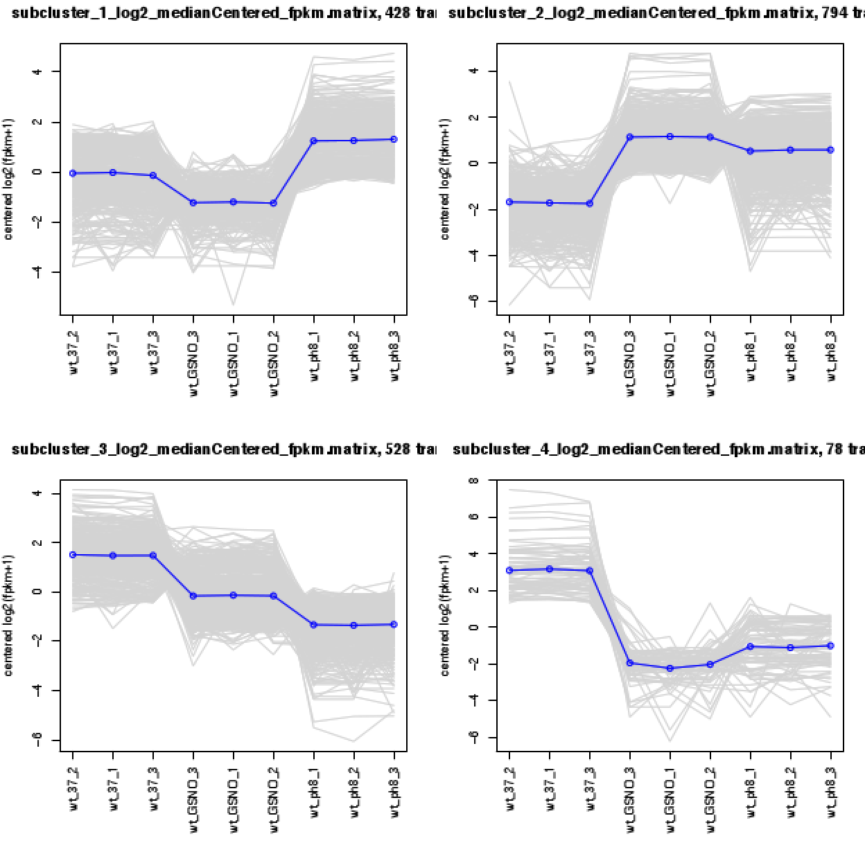
A directory will be created called: 'diffExpr.P0.001_C2.matrix.RData.clusters_fixed_P_60' that contains the expression matrix for each of the clusters (log2-transformed, median centered). A summary pdf file is provided as 'my_cluster_plots.pdf' that shows the expression patterns for the genes in each cluster. Each gene is plotted (gray) in addition to the mean expression profile for that cluster (blue), as shown below:
The example data shown here is provided in the Trinity toolkit under:
$TRINITY_HOME/sample_data/test_DE_analysis
and are based on RNA-Seq data generated by this work [“Defining the transcriptomic landscape of Candida glabrata by RNA-Seq”. Linde et al. Nucleic Acids Res. 2015 ] (http://www.ncbi.nlm.nih.gov/pubmed/?term=25586221)
The TM4 MeV application is a desktop application for navigating expression data derived from microarrays or RNA-Seq data.
Visit our Trinity documentation for using MeV for an introductory guide on how to navigate your DE transcript or gene matrices.
It can be useful to include functional annotations (eg. transporter) to the transcript or gene identifiers in your expression matrix, particularly when exploring your expression data using tools such as MeV as described above.
If you ran Trinotate to functionally annotate your transcriptome, then you can do the following to encode the functional annotation information into the feature name column of your matrix. Note, this uses software in both Trinotate and Trinity, so examine the commands below carefully.
First, convert your Trinotate.xls annotation file into a feature name annotation mapping file where each feature name (gene or transcript ID) is mapped to a version that has functional annotations encoded within it.
${TRINOTATE_HOME}/util/Trinotate_get_feature_name_encoding_attributes.pl \
        Trinotate_report.xls > Trinotate_report.xls.name_mappings
Example output would look like so:
TRINITY_DN986_c0_g2	TRINITY_DN986_c0_g2^PMA2_SCHPO^Cation_ATPase_N^Tm2
TRINITY_DN986_c0_g2_i1	TRINITY_DN986_c0_g2_i1^PMA2_SCHPO^Cation_ATPase_N^Tm2
TRINITY_DN987_c0_g1	TRINITY_DN987_c0_g1^EF3_SCHPO^ABC_tran
TRINITY_DN987_c0_g1_i1	TRINITY_DN987_c0_g1_i1^EF3_SCHPO^ABC_tran
TRINITY_DN987_c0_g2	TRINITY_DN987_c0_g2^EF3_SCHPO^ABC_tran
TRINITY_DN987_c0_g2_i1	TRINITY_DN987_c0_g2_i1^EF3_SCHPO^ABC_tran
TRINITY_DN988_c0_g1	TRINITY_DN988_c0_g1^RAD5_SCHPO^HIRAN
TRINITY_DN988_c0_g1_i1	TRINITY_DN988_c0_g1_i1^RAD5_SCHPO^HIRAN
TRINITY_DN988_c0_g2	TRINITY_DN988_c0_g2^RAD5_SCHPO^UBA_4
TRINITY_DN988_c0_g2_i1	TRINITY_DN988_c0_g2_i1^RAD5_SCHPO^UBA_4
TRINITY_DN989_c0_g1	TRINITY_DN989_c0_g1^YL39_SCHPO^DnaJ
TRINITY_DN989_c0_g1_i1	TRINITY_DN989_c0_g1_i1^YL39_SCHPO^DnaJ
TRINITY_DN989_c0_g2	TRINITY_DN989_c0_g2^YL39_SCHPO^DnaJ
TRINITY_DN989_c0_g2_i1	TRINITY_DN989_c0_g2_i1^YL39_SCHPO^DnaJ
TRINITY_DN98_c0_g1	TRINITY_DN98_c0_g1^GET4_SCHPO^DUF410^sigP
TRINITY_DN98_c0_g1_i1	TRINITY_DN98_c0_g1_i1^GET4_SCHPO^DUF410^sigP
Then, update your expression matrix to incorporate these new function-encoded feature identifiers:
${TRINITY_HOME}/Analysis/DifferentialExpression/rename_matrix_feature_identifiers.pl \
  Trinity_trans.TMM.EXPR.matrix Trinotate_report.xls.name_mappings  > Trinity_trans.TMM.EXPR.annotated.matrix