QC Samples and Biological Replicates
Once you've performed transcript quantification for each of your biological replicates, it's good to examine the data to ensure that your biological replicates are well correlated, and also to investigate relationships among your samples. If there are any obvious discrepancies among your sample and replicate relationships such as due to accidental mis-labeling of sample replicates, or strong outliers or batch effects, you'll want to identify them before proceeding to subsequent data analyses (such as differential expression).
The Trinity toolkit includes a script 'PtR' (pronounced Peter, and stands for Perl-to-R) that can be used to generate a variety of plots for exploring your matrix of expression data. We'll be using it in each of the steps below. You'll be needing the following two files to proceed:
-
your fragment counts matrix, which we'll call 'counts.matrix' generated by the earlier abundance estimation routines.
-
a 'samples.txt' file, with tab-delimited format:
 condition_A_name     replicate_A1_name
 condition_A_name     replicate_A2_name

 condition_B_name     replicate_B1_name
 condition_B_name     replicate_B2_name
and the replicate names should match identically to the column headers of your 'TMM.EXPR.matrix' and 'counts.matrix' files.
Below we demonstrate the use of PtR on data derived from RNA-Seq generated in this paper: [“Defining the transcriptomic landscape of Candida glabrata by RNA-Seq”. Linde et al. Nucleic Acids Res. 2015 ] (http://www.ncbi.nlm.nih.gov/pubmed/?term=25586221), with an example counts matrix provided in the Trinity toolkit at $TRINITY_HOME/sample_data/test_DE_analysis
Run PtR like so to compare the biological replicates for each of your samples.
  % $TRINITY_HOME/Analysis/DifferentialExpression/PtR --matrix counts.matrix \
                  --samples samples.txt --log2 --CPM \
                  --min_rowSums 10 \
                  --compare_replicates
Here, PtR reads in the matrix of counts, performs a counts-per-million (CPM) data transformation followed by a log2 transform, and then generates a multi-page pdf file (named ${sample}.rep_compare.pdf) for each of your samples, including several useful plots:
After running PtR as above, run 'ls -ltr' in your terminal, which will list all files in your working directory with newest files at the bottom. Here you should see the newly output *.pdf files. View the pdf files to examine the plots.
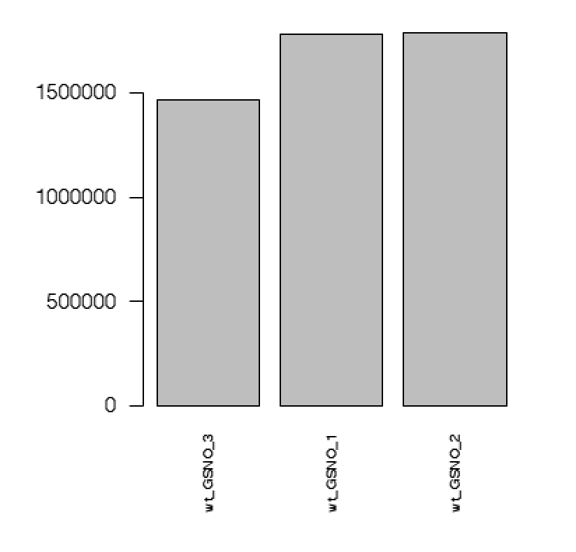
A plot showing the sum of mapped fragments:
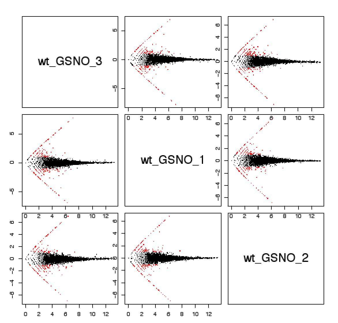
Pairwise comparisons of replicate log(CPM) values. Data points more than 2-fold different are highlighted in red:

Pairwise MA plots (x-axis: mean log(CPM), y-axis log(fold_change)):
and a replicate Pearson correlation heatmap:

Now let's compare replicates across all samples. Run PtR to generate a correlation matrix for all sample replicates like so:
 %  $TRINITY_HOME/Analysis/DifferentialExpression/PtR \
          --matrix Trinity_trans.counts.matrix \
          --min_rowSums 10 \
          -s samples.txt --log2 --CPM --sample_cor_matrix
which generates file 'counts.matrix.minCol10.minRow10.log2.sample_cor_matrix.pdf'
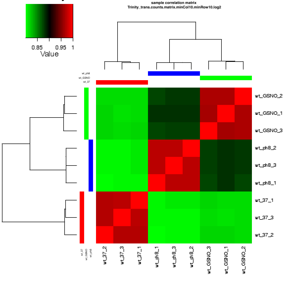
As you can see in the above, the replicates are more highly correlated within samples than between samples.
Another important analysis method to explore relationships among the sample replicates is Principal Component Analysis (PCA). You can generate a PCA plot like so:
 %  $TRINITY_HOME/Analysis/DifferentialExpression/PtR \
    --matrix Trinity_trans.counts.matrix \
    -s samples.txt --min_rowSums 10 --log2 \
    --CPM --center_rows \
    --prin_comp 3
This generates a file 'Trinity_trans.counts.matrix.minRow10.CPM.log2.prcomp.principal_components.pdf'.

The --prin_comp 3 indicates that the first three principal components will be plotted, as shown above, with PC1 vs. PC2 and PC2 vs. PC3. In this example, the replicates cluster tightly according to sample type, which is very reassuring.
If you have replicates that are clear outliers, you might consider removing them from your study as potential confounders. If it's clear that you have a batch effect, you'll want to eliminate the batch effect during your downstream analysis of differential expression.