Sacurine statistical workflow

Univariate hypothesis testing, multivariate modeling, and feature selection

By Etienne Thévenot (last updated: 2017-08-18)

For a video demonstration of the workflow watch webinar Statistical workflows in PhenoMeNal by Etienne Thévenot

Contents

1. Univariate and multivariate analysis of metabolomics data
2. The "W4M univariate-multivariate-statistics" history (W4M00001)
3. Tutorial
   1. Video
   2. Accompanying text with screenhots
4. Interpretation of the results
   1. Principal component analysis (PCA)
   2. Univariate hypothesis testing
   3. Orthogonal Partial Least Squares - Discriminant Analysis (OPLS-DA)
   4. Selection of significant signatures
5. Enjoy your analyses!
   1. Input format
   2. Feedback and help
6. Acknowledgements

1. Univariate and multivariate analysis of metabolomics data

Statistics are a critical step in metabolomics (and the other omics) data analysis, e.g. to:

1. explore the dataset (visualize the data, detect outlier samples or variables, identify cluster of samples)
2. identify which variables have intensities signficantly distinct between levels of qualitative factor (or are signficantly correlated with a quantitative response)
3. build predictive models of these responses
4. select variables which significantly contribute to the performance of these models

Three modules have been developed in Galaxy to perform such statistics:

• univariate for step 2
• multivariate (Wold, 2001; Trygg and Wold, 2002; Thévenot et al, 2015) for steps 1 (Principal Component Analysis) and 3 (Partial Least-Squares)
• biosigner (Rinaudo et al, 2016) for step 4 (significant signatures for either Partial Least Square Discriminant Analysis, Random Forest, or Support Vector Machine classifiers between two groups). They are available on the Workflow4Metabolomics e-infrastructure (Guitton et al, 2017), and also on the PhenoMeNal instance as described in the tutorial below.

These analyses take a input a sample by variable table of intensities (e.g. an MS peak table, or an NMR table of bucket intensities) in addition to, for steps 2-3, the values of the response (e.g. treatment, body mass index, etc.). They return metrics about samples (e.g. scores) or variables (e.g. p-values, loadings, Variable Importance in Projection).

Back to "Contents"

2. The "W4M univariate-multivariate-statistics" history (W4M00001)

This history, which is publicly available on the PhenoMeNal instance, is an example of a statistical workflow applied to metabolomics data. The objective is to characterize the physiological variations of the urine metabolome with age, body mass index (BMI), and gender in a human cohort (Thévenot et al, 2015).

The dataset (named sacurine and available from the MetaboLights repository: MTBLS404) consists of:

1. a peak table of 183 samples and 110 metabolites
2. the age, BMI, and gender of the 183 volunteers

The format of the dataset consists of 3 tables: the dataMatrix, the sampleMetadata, and the variableMetadata tabulated files (.tsv files which you can open with spreadsheet software such as Excel or OpenOffice). More details about these formats can be found on slides 4-9 from this presentation.

The workflow (W4M00001) consists of:

1. Principal Component Analysis (PCA) of the dataset
2. Student's t-test of intensity differences between gender, with correction for multiple testing (False Discovery Rate, FDR)
3. Orthogonal Partial Least Squares - Discriminant Analysis (OPLS-DA) modeling of gender
4. Selection of significant signatures for prediction with either Partial Least Squares - Discriminant Analysis (PLS-DA), Random Forest, or Support Vector Machine (SVM).

Note: More details about this history can be found on the Workflow4Metabolomics platform (W4M00001; DOI:10.15454/1.4811121736910142E12).

Back to "Contents"

3. Tutorial

The purpose of this tutorial is to show you how to import and re-run the history, to better understand how to use the statistical modules for your own analyses.

The history (i.e., the workflow and associated input and ouput data) is only available at our PhenoMeNal public instance.

The tutorial (which you can follow either with the videos or with the accompanying text) shows you how to:

• import the history into your own account,
• extract the workflow,
• modify the workflow input parameters (optionally),
• and run it with either the example data or your own.

Note: if you are new to Galaxy we strongly advise you to first read the "Galaxy 101 - What is Galaxy?" tutorial which will help you get a better understanding about the basic concepts when running workflows in Galaxy.

i) Video

The complete workflow can be viewed in action by watching the following two video tutorials:

STEP 1: How to find and use the Galaxy application

STEP 2: Univariate and Multivariate Statistics workflow tutorial

This video tutorial explains the procedure to load the workflow and match the loaded data to the inputs of the workflow.

Back to "Contents"

ii) Accompanying text with screenhots

Step 1: Register and login

Click on "Login or register" tab on the menu of welcome page of Galaxy instance to enter your username and password. For information on how to obtain an account see How to register.

Note : To extract the workflows and re-run it, please ensure that you are logged in before proceeding to step two. If you proceed without an account you will only be able to view the results of the shared history.

Step 2: Import the history

Go to "Shared Data" on the top menu and click "Histories" from drop-down menu. This will bring you to an overview of histories shared by others.

For this tutorial, select "Univariate and Multivariate Statistics" history. After you click on the link it will give an overview of the dataset.

If all went well, you should see a list of intermediate datasets, all shown on a green background. The last thing we have to do here is click on the "import history" link it the upper right part of the page. This will give you the option to rename the history into something else, or leave it as "imported: ...". Finally click on "Import" to save the history in your own account.

When done correctly, you should see the history appear in the right part of the screen. If so, you can proceed to the next step.

Step 3: Extract the workflow

By now you can view the history, but to run the actual workflow you have to extract it first from this imported history. This is done by clicking on the "History options" button (wheel/gear icon) in the upper right part of the screen, right above the search box. Select the "Extract Workflow" option here.

Same as for the history, you can now change the name of the workflow, and click on the "Create Workflow" button below the name to extract and save the workflow to your account. When done correctly, you should now see a blue bar with some text that allows you to edit or run the workflow.

If so, you can proceed to the next step.

Step 4: Edit the workflow

You are now able to view, edit and run the extracted workflow. In the menu at the top of the page you find an option "Workflow". On that page you can select the extracted workflow from step 3. When you choose the edit option you can change the individual tools and the parameters used when running the workflow. For example you could change the "(Corrected) p-value significance threshold" from 0.05 to 0.01 in the Univariate tool to get more stringent results.

After you make changes to the workflow you have to save them before leaving the "edit" page. This is done by clicking the "Settings" button (wheel/gear icon) in the upper right part of the screen.

Warning: Saving workflows is very important since, unlike histories, workflows are not saved automatically.

Step 5: Run the workflow

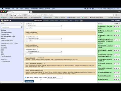
Same as step 4, in the menu at the top of the page you find an option "Workflow". On that page you can select the edited workflow from step 4. But now instead of selecting "edit", we choose "run". This page will allow you to overwrite or create a new history, and select the required input data. Choose a new history, and make sure the "dataMatrix.tsv" is selected in the first input field, "sampleMetaData.tsv" in the second, and "variableMetaData.tsv" in the third. When this is done you can click on "Run workflow", a blue button on the top of the page.

The tools of the workflow will now be scheduled to run as soon as resource become available. In case you selected "Send results to a new history", you will have to switch histories first! This is done using the "View all histories" button in the upper right corner, next to the "History options" button from step 3. Here you can select the correct (newly created) history. You can now follow the progress in the "history" pane on the right. When all boxed are green it finished. You can now view the result of the individual tools by clicking on the "eye"-icon of the appropriate tool.

Step 6: View the results

Now that we have successfully ran an imported history and workflow, we can look at the results. All tools with output will show an "eye"-icon in the green box of the workflow history. This will open/preview the results in Galaxy. Optionally you can edit, download or delete results.

Back to "Contents"

4. Interpretation of the results

Below is a description of some of the ouputs from each module. You can find additional details about the statistical modules (parameters, diagnostics, output files and graphics) in:

• the documentation section at the bottom of the Galaxy pages (where you select your parameters)
• the course presentations on the Workflow4Metabolomics plaform about univariate and multivariate statistics
• the vignettes from the ropls and biosigner R/Bioconductor packages

Back to "Contents"

4.i) Principal component analysis (PCA)

The multivariate module enables to perform either principal component analysis (PCA), partial least-squares (PLS and PLS-DA), and orthogonal partial least-squares (OPLS and OPLS-DA, see section 4.iii).

	Y Response	Number of predictive components	Number of orthogonal components
PCA	none	NA or >0	0
PLS	quantitative column of sampleMetadata	NA or >0	0
PLS-DA	qualitative column of sampleMetadata	NA or >0	0
OPLS	quantitative column of sampleMetadata	1	NA or >0
OPLS-DA	qualitative column of sampleMetadata	1	NA or >0

Here, the Y Response parameter has been set to 'none' in order to perform unsupervised PCA data exploration.

The defaults graphic is shown below (as we are more interested in the gender factor here, we asked to color the points from the score plots by setting Ellipses to gender, in the Advanced graphical parameters). We observe that the difference between genders is not main source of variance in the first two PCA dimensions.

Figure 4.i: PCA summary plot. Top left overview: the scree plot (i.e., inertia barplot) suggests that 3 components may be sufficient to capture most of the inertia; Top right outlier: this graphics shows the distances within and orthogonal to the projection plane (see Hubert et al., 2005): the name of the samples with a high value for at least one of the distances are indicated; Bottom left x-score: the variance along each axis equals the variance captured by each component: it therefore depends on the total variance of the dataMatrix X and of the percentage of this variance captured by the component (indicated in the labels); it decreases when going from one component to a component with higher indice; Bottom right x-loading: the 3 variables with most extreme values (positive and negative) for each loading are black colored and labeled.

Note:

1. A specific Graphic type can be selected within the Advanced graphical parameters [default = summary]

2. Since the dataMatrix does not contain missing value, the singular value decomposition was used by default; NIPALS can be selected with the Algorithm argument within the Advanced computational parameters,

3. The default (NA) Number of predictive components for PCA means that components (up to 10) will be computed until the cumulative variance exceeds 50%. If the 50% have not been reached at the 10th component, a warning message will be issued (you can still compute the following components by specifying the Number of predictive components value).

4. The values of the scores (respectively the loadings) along the two selected components have been added to the [4. Multivariate_sampleMetadata.tsv] (respectively to the [5. Multivariate_variableMetadata.tsv]) tables

5. The values of the variance captured by the 9 components can be seen in the [7. Multivariate_information.txt] text file

Back to "Contents"

4.ii) Univariate hypothesis testing

Forty-one variables (37%) have a significant differences between gender means by using a t-test at a False Discorery Rate (FDR) of 5% ([10. Univariate_information.txt]). As expected, Testosterone glucuronide is significant.

For each variable, we get in the 3 columns added to the variableMetadata file [8. Univariate_Multivariate_variableMetadata.tsv] the values from:

• the difference between gender means (_dif column)
• the corrected p-value (_fdr column)
• the indicator of significance at our input threshold (_sig)

The boxplots from all variables with significant mean difference between genders are available within the [9. Univariate_figure.pdf] file.

Figure 4.ii: Boxplot from all variables with significant mean difference between genders ([9. Univariate_figure.pdf]). Testosterone glucuronide is very significant (corrected p-value < 1e-9; page nb 38). The male volunteer (#38) has a suprisingly low measured concentration.

Back to "Contents"

4.iii) Orthogonal Partial Least Squares - Discriminant Analysis (OPLS-DA)

The Y Response has now been set to the 'gender' qualitative column from the sampleMetadata table, and the Number of orthogonal components to NA, in order to perform Orthogonal Partial Least Squares - Discriminant Analysis (OPLS-DA).

Orthogonal Partial Least Squares (OPLS) is a variant of Partial Least Squares (PLS), which enables to separately model the variation correlated (predictive) to the factor of interest and the uncorrelated (orthogonal) variation (Trygg and Wold, 2002). While performing similarly to PLS, OPLS facilitates interpretation. In addition to scores, loadings and weights plots, the module provides metrics and graphics to determine the optimal number of components (e.g. with the R2 and Q2 coefficients), to check the validity of the model by permutation testing, detect outliers, and provide several metrics to assess the importance of the variables in the model (e.g. Variable Importance in Projection or regression coefficients;). The module is an implementation of the ropls R package available from Bioconductor (Thevenot et al, 2015).

Notes:

1. Overfitting: overfitting (i.e., building a model with good performances on the training set but poor performances on a new test set) is a major caveat of machine learning techniques applied to data sets with more variables than samples. A simple simulation with a random dataMatrix and a random response shows that perfect PLS-DA classification can be achieved as soon as the number of variables exceeds the number of samples. It is therefore essential to check that the Q2 value of the model is significant by random permutation of the labels: the number of permutations (advanced computational parameter) is set to 20 by default but should be increased for confirmation of the results.

2. VIP from OPLS models: the classical VIP metric is not useful for OPLS modeling of a single response. Galindo-Prieto et al, 2014 have therefore recently suggested new VIP metrics for OPLS, VIPpred and VIPortho, to separately measure the influence of the features in the modeling of the dispersion correlated to, and orthogonal to the response, respectively (the 2 metrics are provided as additional columns of the variableMetadata file: [12. Multivariate_Univariate_Multivariate_variableMetadata.tsv]).

3. (Orthogonal) Partial Least Squares Discriminant Analysis: (O)PLS-DA: the approach for discriminant analysis implemented in the module relies on internal conversion of the response into a dummy vector (resp. a matrix when the number of classes is > 2), mean-centering and unit-variance scaling of the vector (resp. the matrix), and PLS (resp. PLS2) regression modeling. When the sizes of the 2 classes are unbalanced, Brereton and Lloyd, 2014 have demonstrated that a bias is introduced in the computation of the decision rule, which penalizes the class with the highest size. In the multiclass case, the proportions of 0 and 1 in the columns is usually unbalanced (even in the case of balanced size of the classes) resulting in a bias (Brereton and Lloyd, 2014). With the current implementation of the module, we thus recommend to stick to binary discrimination and use balanced classes for optimal use.

Figure 4iii: OPLS-DA model of the gender response. Top left: significance diagnostic: the R2Y and Q2Y of the model are compared with the corresponding values obtained after random permutation of the y response; Top right: inertia barplot: the graphic here suggests that 2 orthogonal components may be sufficient to capture most of the inertia; Bottom left: outlier diagnostics; Bottom right: x-score plot: the number of components and the cumulative R2X, R2Y and Q2Y are indicated below the plot.

Notes:

• the NIPALS algorithm is used for PLS (and OPLS); dataMatrix matrices with (a moderate amount of) missing values (typically below 20%) can thus be analysed.
• for OPLS(-DA) modeling of a single response, the number of predictive component is 1
• in the (x-score plot), the predictive component is displayed as abscissa and the (selected; default = 1) orthogonal component as ordinate.

We see that our model with 2 orthogonal components has significant and quite high R2Y and Q2Y values ([13. Multivariate__figure.pdf]).

Back to "Contents"

iv) Selection of significant signatures

Principle

The biosigner module, based on the biosigner R/Bioconductor package, implements an innovative method to select variables which significantly contribute to the prediction performance of a binary classifier (i.e. for the discrimination between two classes; Rinaudo et al., 2016): a group of variables is significant if the prediction performance of the classifier decreases when the values of these variables are permutated in a test subset.

The procedure is repeated iteratively by applying the algorithm to the dataset restricted to the significant variables until, for a given round, all candidate variables are found significant (in this case the signature consists of these variables), or until there is no variable left to be tested (in this case the signature is empty). The biosigner module therefore returns a stable final S signature (possibly empty), in addition to several tiers (from A to E) corresponding to the variables discarded during one of the previous iterations (e.g., variables from the A tier were selected in all but the last iteration).

Because test subsets are generated by a random process (bootstrap), the module may generate slightly distinct signatures when re-applied to the same input data. Fixing the Seed in the Advanced computational parameters ensures that results will be identical.

Signatures from three distinct classifiers can be run in parallel, namely Partial Least Square Discriminant Analysis (PLS-DA), Random Forest (RF) and Support Vector Machines (SVM), as the performances of each machine learning approach may vary depending on the structure of the dataset. The signature for each of the selected classifier(s) as an additional column of the variableMetadata table ([15. Biosigner_Multivariate_Univariate_Multivariate_variableMetadata.tsv]). In addition the tiers and individual boxplots of the selected features are plotted (see below).

The module has been successfully applied to transcriptomics and metabolomics data (Rinaudo et al., 2016).

Notes:

1. only binary classification is currently available
2. if the dataMatrix contains missing values (NA), these features will be removed prior to modeling with Random Forest and SVM (in contrast, the NIPALS algorithm from PLS-DA can handle missing values)

Application to the MTBLS404 "sacurine" dataset

Signatures consisting of 2 (Random Forest) or 3 (PLS-DA, SVM) metabolites (i.e., less than 3% of the initial features) were identified by biosigner ([16: Biosigner__figure-tier.pdf]). Testosterone glucuronide was common to all 3 signatures, and oxoglutaric acid and p-anisic acid to 2 of them. All selected metabolites had a clearcut difference of intensities between males and females ([17: Biosigner__figure-boxplot.pdf]). Prediction accuracies of the models restricted to the signatures (3% of the initial variables) were almost as good as (and superior to for PLS-DA) the models trained on the full dataset ([18: Biosigner__information.txt]).

Figure 4.iv: 4Selected variables from the dataset for the PLS-DA, Random Forest, or SVM prediction of gender. The S tier corresponds to the final metabolite signature, i.e., metabolites which passed through all the selection steps.

Back to "Contents"

5. Enjoy your analyses!

Thank you for working your way through the tutorial and enjoy further analyses with your own data.

5.i) Input format

The format of the dataset consists of 3 tables: the dataMatrix, the sampleMetadata, and the variableMetadata tabulated files (.tsv files which you can open with spreadsheet software such as Excel or OpenOffice). The column names of the dataMatrix (sample names) must be exactly the same as the row names of the sampleMetadata. The row names of the dataMatrix (variable names) must be exactly the same as the row names of the variableMetadata. Please use alphanumerical characters ([0-9], [a-z], [A-Z]) and '_' only in your sample and variable names, without blanks. No specific column name is required in the sampleMetadata (which should contain your factors of interest for the statistics). The 3 tables must have at least 1 column (in addition to the row names). More details about these formats can be found on slides 4-9 from this presentation.

5.ii) Feedback and help

Feel free to report any feedback to us by email or via the Online Feedback Form.

Other tutorials are available on our website (see the PhenoMeNal wiki).

Back to "Contents"

6. Acknowledgements

All of these Galaxy modules have been containerized by Pierrick Roger and integrated into the PhenoMeNal instance with the help of Pablo Moreno. Michael van Vliet did a huge work in improving and testing this tutorial.

Back to "Contents"