Brief Introduction

This tutorial is meant to help you get started with writing you own C# applications using the Platform for Situated Intelligence (or \psi). Some of the topics that are touched upon here are explained in more depth in other documents.

The tutorial is structured in the following easy steps:

1. A simple \psi application - describes first steps in creating a very simple \psi application.
2. Synchronization - describes how to fuse and synchronize multiple streams.
3. Saving Data - explains how to persists streams to disk.
4. Replaying Data - explains how to replay data from a persisted store.
5. Visualization - explains how to use Platform for Situated Intelligence Studio (PsiStudio) to visualize persisted streams, or live streams from a running \psi application.
6. Further Reading - provides pointers to further in-depth topics.

1. A simple \psi application

Before writing up our first \psi app, we will need to setup a Visual Studio project for it. Follow these steps to set it up:

1. First, create a simple .NET Core console app (for the examples below, a console app will suffice). You can do so by going to File -> New Project -> Visual C# -> Console App (.NET Core). (.NET Core is a cross-platform solution; if you want to createa .NET Framework solution which runs only on Windows, make sure you change your project settings to target .NET Framework 4.7 or above.)

2. Add a reference to the Microsoft.Psi.Runtime NuGet package that contains the core Platform for Situated Intelligence infrastructure. You can do so by going to References (under your project), right-click, then Manage NuGet Packages, then go to Browse. Make sure the Include prerelease checkbox is checked. Type in Microsoft.Psi.Runtime and install. Under Linux, this can be accomplished by dotnet new console -n BriefIntro && cd BriefIntro and dotnet add package Microsoft.Psi.Runtime.

3. As the final step, add a using clause at the beginning of your program as follows:

using Microsoft.Psi;

You are now ready to start writing your first \psi application!

A \psi application generally consists of a computation graph that contains a set of components (nodes in the graph), connected via time-aware streams of data (edges in the graph). Most \psi applications use various sensor components (like cameras, microphones) to generate source streams, which are then further processed and transformed by other components in the pipeline. We will start simple though, by creating and displaying a simple source stream: a timer stream that posts messages every 100 ms.

To do so, we start by creating the pipeline object, which represents and manages the graph of components that make up our application. Among other things, the pipeline is responsible for starting and stopping the components, for running them concurrently and for coordinating message passing between them. To create the pipeline, we use the Pipeline.Create factory method, like below:

static void Main(string[] args)
{
    using (var p = Pipeline.Create())
    {
    }
}

Now, let's add the logic for constructing the timer stream, and for displaying the messages on it:

static void Main(string[] args)
{
    using (var p = Pipeline.Create())
    {
        var timer = Timers.Timer(p, TimeSpan.FromSeconds(0.1));
        timer.Do(t => Console.WriteLine(t));
        p.Run();
    }
}

Try it out!

The Timers.Timer factory method creates a source timer stream. In this case, the first parameter in the call is the pipeline object p (a common pattern in \psi when instantiating components) and the second parameter is the time interval to use when generating messages is specified as the second parameter.

Streams are a fundamental construct and a first-order citizen in the \psi runtime. They can be generated and processed via various operators and they link components together. Streams are a generic type (you can have a stream of any type T) and are strongly typed, and therefore the connections between components are statically checked. Messages posted on streams are time-stamped and streams can be persisted to disk and visualized (more on that in a moment).

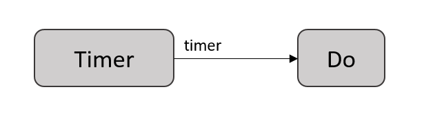
In the example above Do() is a stream operator, which executes a function for each message posted on the stream. In this case, the function is specified inline, via an anonymous delegate t => Console.WriteLine(t) and simply writes the message to the console. Under the covers, each stream operator is backed by a component: the Do() extension method creates a Do component that subscribes to the Timer component. In reality, the pipeline we have just constructed looks like this:

The delegate passed to the Do operator takes a single parameter, which corresponds to the data arriving on the stream. Another overload of the Do operator also gives access to the message envelope, which contains the time-stamp information. To see how this works, change the timer.Do line in the example above to:

timer.Do((t, e) => Console.WriteLine($"{t} at time {e.OriginatingTime.TimeOfDay}"));

This time the timestamp for each message will be displayed. You may notice that the timestamps don't correspond to your local, wall-clock time. This is because \psi messages are timestamped in UTC.

The p.Run() line simply runs the pipeline. A number of overloads and other (asynchronous) methods for running the pipeline are available, but for now, we use the simple Run() method which essentially tells the pipeline to execute to completion. This causes the generator to start generating messages, which in turn are processed by the Do operators. Since the generator outputs a timer stream that is infinite this application will continue running indefinitely until the console is closed by the user.

There are many basic, generic stream operators available in the \psi runtime (for an overview, see Basic Stream Operators, and also operators for processing various types of streams (like operators for turning a stream of color images into a corresponding stream of grayscale images). Besides Do, another operator that is often used is Select. The Select operator allows you to transform the messages on a stream by simply applying a function to them. Consider the example below (you will have to also add a using System.Linq; directive at the top of your program to access the Enumerable class):

static void Main(string[] args)
{
    using (var p = Pipeline.Create())
    {
        var sequence = Generators.Sequence(p, 0d, x => x + 0.1, 100, TimeSpan.FromMilliseconds(100));
        sequence
            .Select(t => Math.Sin(t))
            .Do(t => Console.WriteLine($"Sin: {t}"));
        p.Run();
    }
}

Before we discuss the Select, note that we have used a different generator this time to create a source stream that outputs a sequence of values. The Generators.Sequence factory method creates a stream that posts a sequence of messages. In this particular case the sequence is specified via an initial value (0d), an update function (x => x + 0.1) and a total count of messages to be generated (100). The messages will be posted at 100 millisecond intervals. Note also that in this case, when we run the pipeline, the sequence and hence the source stream is finite, and as a result the pipeline will complete and the program will exit once the end of the sequence is reached.

The Select operator we have injected transforms the messages from the sequence stream by computing the sine function over the messages. Try this and check out the results! You should see in the console a sequence of outputs that fluctuate between -1 and +1, like the sinus function.

Beyond Do and Select, \psi contains many operators: single stream operators like Where, Aggregate, Parallel etc. (similar with Linq and Rx), stream generators (Sequence, Enumerate, Timer) as well as operators for combining streams (Join, Sample, Repeat). Like Do, some of these operators also have overloads that can surface the message envelope information. Check out the Basic Stream Operators page for an in-depth look at all of them.

Finally, so far we have highlighted the language of stream operators, which encapsulate simple components that perform transformations on streams. In the more general case, \psi components can have multiple inputs and outputs and can be wired into a pipeline via the PipeTo operator. For instance, in the example below we instantiate a wave file audio source component, and connect its output to an acoustic features extractor component, after which we display the results. For the below sample, be sure to add a reference to the Microsoft.Psi.Audio NuGet package (under Linux, dotnet add package Microsoft.Psi.Audio).

using (var p = Pipeline.Create())
{
    // Create an audio source component
    var waveFileAudioSource = new WaveFileAudioSource(p, "sample.wav");

    // Create an acoustic features extractor component
    var acousticFeaturesExtractor = new AcousticFeaturesExtractor(p);

    // Pipe the output of the wave file audio source component into the input of the acoustic features extractor
    waveFileAudioSource.Out.PipeTo(acousticFeaturesExtractor.In);

    // Process the output of the acoustic features and print the messages to the console
    acousticFeaturesExtractor.SpectralEntropy.Do(s => Console.WriteLine($"SpectralEntropy: {s}"));
    acousticFeaturesExtractor.LogEnergy.Do(e => Console.WriteLine($"LogEnergy: {e}"));

    // Run the pipeline
    p.Run();
}

Writing a \psi application will often involve authoring a pipeline that connects various existing components and processes and transforms data via stream operators. In some cases, you may need to write your own components. The Writing Components page has more in-depth information on this topic. In addition, to optimize the operation of your pipeline, you may need to specify delivery policies to control how messages may be dropped in case some of the components cannot keep up with the cadence of the incoming messages. The Delivery Policies page has more in-depth information on this topic.

2. Synchronization

Building systems that operate over streaming data often requires that we do stream-fusion, i.e., join data arriving on two different streams to form a third stream. Because execution of the various components in a \psi pipeline is asynchronous and parallel, synchronization becomes paramount, i.e., how do we match (or pair-up) the messages that arrive on the different streams to be joined?

The answer lies in the fact that \psi streams are time-aware: timing information is carried along with the data on each stream, enabling both the developer and the runtime to correctly reason about the timing of the data. Specifically, the way this works is that the data collected by sensors (the data on source streams) is timestamped with an __originating time that captures when the data captured by the sensor occured in the real world. For instance, messages posted on the output stream of the video camera components will time-stamp each frame with the originating time of when that image frame was collected by the sensor. As the image message is processed by a downstream ToGray() component, the originating time is propagated forward on the resulting grayscale image message. This way, a downstream component that receives the grayscale image will know what was the time of this data in the real world. And, if the component has to fuse information from the grayscale image with results from processing an audio-stream (which may arrive at a different latency), because the component has access to originating times on both streams, it can reason about time and pair the streams.

To facilite this type of synchronization \psi provides a special Join stream operator that allows you to fuse multiple streams and control the synchronization mechanism used in this process.

To illustrate this, let's look at the following example:

using (var p = Pipeline.Create())
{
    var sequence = Generators.Sequence(p, 0d, x => x + 0.1, 100, TimeSpan.FromMilliseconds(100));

    var sin = sequence.Select(t => Math.Sin(t));
    var cos = sequence.Select(t => Math.Cos(t));

    var joined = sin.Join(cos);
    joined.Do(m =>
    {
        var (sinValue, cosValue) = m;
        Console.WriteLine($"Sum of squares: {(sinValue * sinValue) + (cosValue * cosValue)}");
    });
    p.Run();
}

The example computes two streams, containing the sin and cos values for the original sequence. The streams are then joined via the join operator: sin.Join(cos). The join operator synchronizes the streams: the messages arriving on the sin and cos streams are paired based on matching originating times. The Join operator produces an output stream containing a C# tuple of double values, i.e. (double, double) - you can see this by hovering over the joined variable in Visual Studio. This is generally the case: when joining two streams of type TA and TB, the output stream will be a tuple of (TA,TB).

Try the example out! You should be getting a printout that looks like:

Sum of squares: 1.0000
Sum of squares: 1.0000
Sum of squares: 1.0000
Sum of squares: 1.0000

The answer is always one. Yes, Pythagora's theorem still holds: sin ^ 2 + cos ^ 2 = 1. But there is in fact something more interesting going on here that we would like to highlight. The reason we get the correct answer is because the Join operator does the proper synchronization and pairs us the messages with the same originating time, regardless essentially of when they arrive (this is important because all the operators execute concurrently respective to each other). The pipeline from the example above contains 5 components, like this:

All of these components execute concurrently. The generator publishes the values, and these are sent to the two Select operators. These two operators publish independently the values computed but maintain the originating time on the messages that get sent downstream. The join operator receives the messages on two different streams. Because of concurrent execution, we do not know the relative order that the messages arrive over the two streams at the Join operator. For instance, one of the computations (say cosinus) might take longer which may create a larger latency (in wall clock time) on that stream. However, because originating times are carried through, Join can pair the messages correctly and hence the sin ^ 2 + cos ^ 2 = 1 equality holds over the output.

To more vividly demonstrate what would happen without this originating-time based synchronization, modify the join line like below:

var joined = sin.Pair(cos);

Re-run the program. This time, the results are not always 1. In this case we have used a different operator, Pair that does not actually reason about the originating times but rather pairs each message arriving on the sin stream with the last message that was delivered on the cos stream. Because of asynchronous execution of operators in the pipeline, this time the pairing might not correspond to the a match in the originating times and in that case the result from summing up the squares is different from 1.

We have illustrated above how to do an exact join (the originating times must match exactly for the messages to be paired). There are many ways to do originating-time based synchronization, with important consequences for the behavior of the pipeline. In this introductory guide, we limit this discussion here, but we recommend that you read the more in-depth topic on the Stream Fusion and Merging page.

3. Saving Data

While the examples provided so far operate with synthetic data for simplicity, this is not generally the case. Usually, the data is acquired from sensors or external systems otherwise connected to the real world. In most cases we want to save the data for analysis and replay. \psi provides a very simple way of doing this, as illustrated in the following example:

using (var p = Pipeline.Create())
{
    // Create a store to write data to (change this path as you wish - the data will be stored there)
    var store = PsiStore.Create(p, "demo", "c:\\recordings");

    var sequence = Generators.Sequence(p, 0d, x => x + 0.1, 100, TimeSpan.FromMilliseconds(100));

    var sin = sequence.Select(t => Math.Sin(t));
    var cos = sequence.Select(t => Math.Cos(t));

    // Write the sin and cos streams to the store
    sequence.Write("Sequence", store);
    sin.Write("Sin", store);
    cos.Write("Cos", store);

    Console.WriteLine("Program will run for 10 seconds and terminate. Please wait ...");
    p.Run();
}

The example creates and saves the sequence and sin and cos streams of double values. This is done by creating a store component with a given name and folder path via the PsiStore.Create factory method, and then using it with the Write stream operator. The store component knows how to serialize and write to disk virtually any .Net data type (including user-provided types) in an efficient way.

The data is written to disk in the specified location (in this case c:\recordings, in a folder called demo.0000. The PsiStore.Create API creates this folder and increases the counter to demo.0001, demo.0002 etc. if you run the application repeatedly. Inside the demo.0000 folder you will find Catalog, Data and Index files. Together, these files constitute the store.

4. Replaying Data

Data written to disk in the manner described above can be played back with similar ease and used as input data for another \psi application. Assuming that the example described in the Saving Data section was executed at least once, the following code will read and replay the data, computing and displaying the sin function.

using (var p = Pipeline.Create())
{
    // Open the store
    var store = PsiStore.Open(p, "demo", "c:\\recordings");

    // Open the Sequence stream
    var sequence = store.OpenStream<double>("Sequence");

    // Compute derived streams
    var sin = sequence.Select(Math.Sin).Do(t => Console.WriteLine($"Sin: {t}"));
    var cos = sequence.Select(Math.Cos);

    // Run the pipeline
    p.Run();
}

An existing store is opened with the PsiStore.Open factory method, and streams within the store can be retrieved by name using the OpenStream method (you will have to know the name and type of the stream you want to access). The streams can then be processed as if they were just generated from a source.

This method of replaying data preserves the relative timing and order of the messages, and by default plays back data at the same speed as it was produced. When you run the program, you will see the Sin values being displayed by the Do operator.

We can control the speed of the execution of the pipeline, via a replay descriptor parameter passed to the Run() method. If noparameter is specified the pipeline uses the ReplayDescriptor.ReplayAllRealTime, which plays back the data at the same speed as it was produced. Try replacing the call to p.Run() with p.Run(ReplayDescriptor.ReplayAll). In this case, the data will play backfrom the store at maximum speed, regardless of the speed at which it was generated. Running the program will display the Sin values much faster now. Note that the originating times are nevertheless preserved on the messages being replayed from the store.

5. Visualization

Visualization of multimodal streaming data plays a central role in developing multimodal, integrative-AI applications. Visualization scenarios in \psi are enabled by the Platform for Situated Intelligence Studio (which we will refer to in short as PsiStudio)

Notes:

• Currently, PsiStudio runs only on Windows, although it can visualize data stores created by \psi applications running on any platform supported by .NET Core.
• The tool is not currently shipped as an executable, so to use it you will need to build the codebase; instructions for building the code are available here. The tool is implemented by the Microsoft.Psi.PsiStudio project in the Psi.sln solution tree under Sources\Tools\PsiStudio. To run it, simply run this project after building it.

PsiStudio enables compositing multiple visualizers of different types (from simple streams of doubles to images, depth maps, etc.). In this section we will give a very brief introduction to this tool.

Now start up PsiStudio. You will see a window that looks similar to the image below.

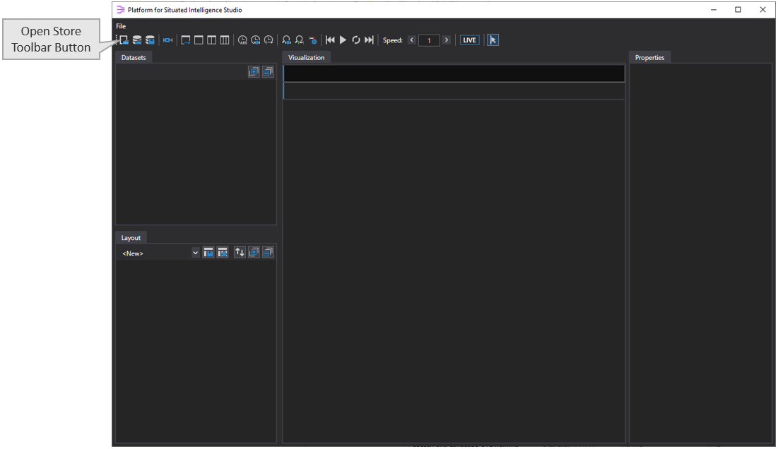
To open a store, click the Open Store toolbar button and navigate to the location you have specified in the example above, e.g. C:\recordings\demo.#### (the last folder corresponds to the last run) and open the Catalog file, e.g. C:\recordings\demo.####\demo.Catalog_000000.psi. The PsiStudio window should now look like this:

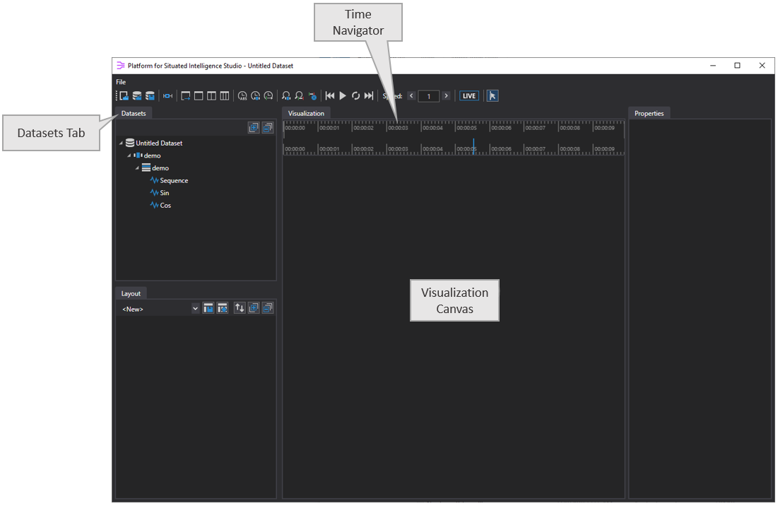
Notice that PsiStudio has created a dataset named Untitled Dataset, then added a session named demo to the dataset, and then added a partition also named demo to the session. This partition represents the store that was created earlier and as you can see it contains all of the streams in that store. A PsiStudio dataset can contain any number of sessions, and each session can contain any number of partitions. More information about datasets, sessions, and partitions is available in the Datasets page.

If you drag the Sin stream from the Datasets tab onto the Visualization Canvas, PsiStudio should now look like this:

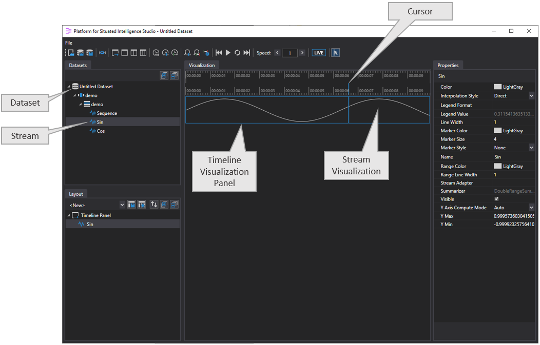
PsiStudio has created a timeline visualization panel and inside it a visualizer for the Sin stream. Moving the mouse over the panel moves the data cursor (which is synchronized across all panels).

If we now drag the Cos stream from the Datasets tab into this same visualization panel, a visualizer for this stream will be overlaid on the current timeline panel, resulting in a visualization like this :

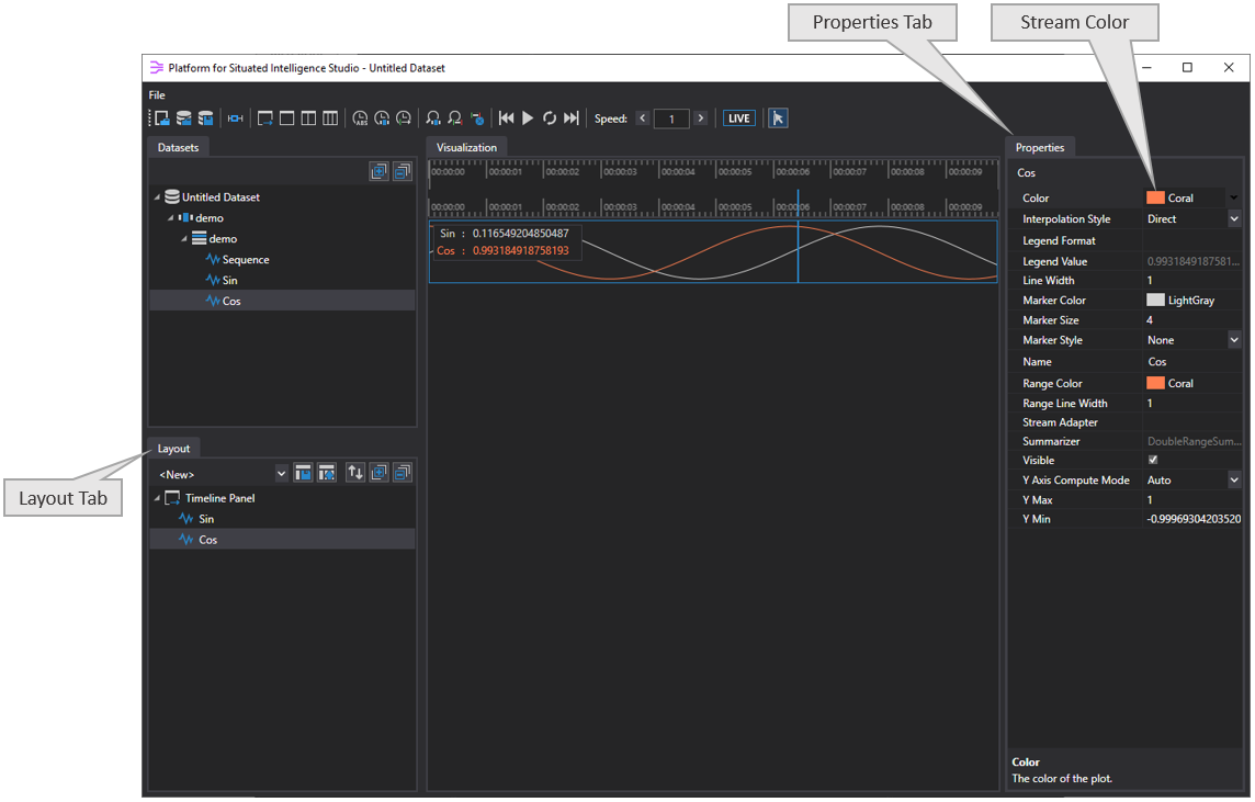
To display the legend that's visible in the image above, simply right click on the timeline panel and select Show/Hide Legend. In order to distinguish between the two streams, we should change the color of one of them. To do this, click on the Cos stream in the Layout tab, this will display the properties of the visualizer that's being used to display the stream in the visualization canvas in the Properties tab on the right. Then you can click on the Color property to change the color of the stream, in this case we've selected Coral.

You will notice that as you move the cursor around over the timeline panel, the legend updates with the current values under the cursor. Navigation can be done via mouse: moving the mouse moves the cursor, and the scroll wheel zooms the timeline view in and out. As you zoom in, you will notice that the time navigator visuals change, to indicate where you are in the data (the blue region in the top-half). You can also drag the timeline to the left or right to view earlier or later data in the stream.

Above we dragged the Cos stream into the panel that contained the Sin stream so that both streams were overlaid. Take a look at the Layout tab on the left, notice that currently there is a single timeline panel containing visualizers for both the Sin and the Cos streams. Suppose however that we wanted to visualize the Cos stream in a different panel.

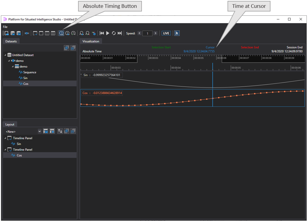
In the Layout tab, right-click on the Cos visualizer to bring up the context-menu and select Remove to remove the Cos stream from the panel. Now go back to the Datasets tab and drag the Cos stream into the empty space below the visualization panel that contains the Sin stream. PsiStudio will create a new visualization panel and add the Cos stream to it.

Now change the Color property of the Cos stream to Coral again, use the mouse wheel to zoom in, and then set the Marker Style property to Square. This will display a small marker at every message in the stream.

Finally, click on the Absolute Timing toolbar button to display some timing information. With this button enabled, the absolute time at the cursor is displayed as you move the cursor around the visualization canvas.

PsiStudio has many more features than what has been covered here, including complex 2D and 3D visualizers and also multi-track annotations. For example, in the image below, PsiStudio was used to visualize a variety of streams from a \psi application that attempts to identify the objects that someone points to in a room.

A much deeper dive into the capabilities of PsiStudio is available here.

6. Next steps

In addition to this brief introduction, a collection of Tutorials is available, that describe in more details various aspects of the framework. These include tutorials on how to write components, on how to control pipeline execution and delivery policies, on basic stream operators available in the framework, as well as operators for stream fusion and merging, interpolation and sampling, windowing, and stream generation.

A number of other, specialized topics are collected under the Other Topics page, including how to create distributed \psi applications via remoting, how to bridge to Python, JS, ... or ROS, shared objects and memory management, etc.

Finally, it may be helpful to look through the set of Samples provided. While some of the samples address specialized topics like how to leverage speech recognition components or how to bridge to ROS, reading them will give you more insights into programming with Platform for Situated Intelligence. In addition, some of the samples have a corresponding detailed walkthrough that explains how the samples are constructed and function, and provide further pointers to documentation and learning materials. Going through these walkthroughs can also help you learn more about programming with \psi.