Indexing 1T vectors
This is a case study on how to index 1.5T vectors. 1 trillion is 1000 billion vectors. Because it is so large scale, we did not do a grid search on parameters to select the best type of index. Instead we run small-scale experiments to validate the approach before building the final index in one pass.
We are given a database of 1.5T vectors of 144 dimensions. The vectors are already quantized with a scalar quantizer to 1 uint8 per component (ie. the vectors occupy 144 bytes).
The context is quite specific because the requirements are unusual:
- storage is on disk instead of in RAM. Flash vs. spinning disk can be discussed, but we cannot afford to put the index in RAM.
- we search the vectors with a fixed range rather than by k-nearest neighbors.
- a latency of < 1 min per query is acceptable, ie. a user can wait for the query to finish.
- given the L2 distance ground-truth, a high precision and recall are required. Recall 99.9%: almost no near vector should be missed. Precision 90%: a post-verification on the descriptors can be applied, but since it is expensive, it should not be fed with too many false positives.
The index needs to be a variant of IndexIVF. IndexIVF partitions vectors into subsets. At search time, only a small number (nprobe) of subsets is visited, and the query vector is compared sequentially to all vectors those subsets. The vectors are (optionally) compressed with some lossy vector codec.
Thus we need to choose how to partition first, then choose a codec.
To evaluate our choice of an index, we work on a sample of 50M queries and 50M database vectors. These sets are de-duplicated. This is 1/30,000 th the scale at which we will operate eventually. We compute the ground-truth matches for the given threshold r. To compute the ground-truth, we use a mix of GPU and CPU Faiss. GPU is convenient because matching 50M to 50M vectors is slow. However, it does not support range search. Therefore we do a k-NN search with k=1024 on GPU, and use CPU Faiss only for the queries where the 1024'th neighbor is at distance < r.
The data is partitioned into K subsets. Each subset is defined by a centroid K. A vector is assigned to the closest centroid and added to that subset. The larger the index, the larger K should be in order to keep the sizes of subsets relatively small.
We evaluated two partitions of the dataset:
-
a simple k-means on the dataset with K=1M or K=10M clusters. We developed a distributed k-means for the 10M cluster case. To efficiently find the nearest centroid to this many centroids we use an
IndexHNSW. In the high-accuracy regime, we found it useful to increase the default settings of HNSW toefConstruction=200 andefSearch=1024. -
the inverted multi-index quantizer (IMI). The clusters are defined as a Cartesian product of two sets of centroids, which helps to increase K quickly. For example, 2x13 means the Cartesian product of 2 sets of 2^13 subsets (K=2^26 = 67.1M centroids). For this use case we also experiment with 3 sets of centroids (3x10, K=1.1B centroids).
We evaluate the partitions on our 50M test set, without encoding the vectors (IndexIVFFlat). Therefore, the precision is always 100%: all vectors found closer than 48 are correct, but we may miss some vectors (as measured by the recall).
The table below shows some statistics on the partitions:
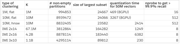
Some subsets are empty because 50M vectors in our test set is a bit small. Here we count the number of non-empty subsets, and the size of the largest cluster. We measure the quantization time for brute-force assignment (flat) on GPU for speed. In practice, we cannot afford a GPU for that, so we use HNSW, which has some impact on accuracy.
We observe that the IMI variants are cheap to assign to and require a very small nprobe to attain a high recall. However, when looking at the size of the subsets, we see that the largest one is usually larger than for the 1M and 10M variants. This is a problem: what's the point of visiting few subsets if the subsets are too large? To evaluate the tradeoff, we measure how many distances should be computed to get a certain recall when varying the nprobe:
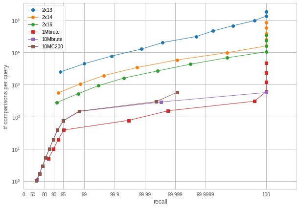
(Number of comparisons required to obtain a certain recall. Note the unusual scaling on the x-axis)
So this tells a different story: IMI is actually worse in terms of number of distance computations. We already observed this, but not in the high-accuracy regime.
For this case, we chose to use 10M centroids. This is more flexible than 1M. For 1.5T vectors, this means there are 150k vectors to visit per centroid on average if the index was balanced (which is not exactly the case, as we will see later).
When stored at full size, the vectors takes 144 bytes per vector (+ 8 bytes for the id). This is too big, so we are going to evaluate if some lossy compression would be acceptable.
Faiss offers several encoding options, see here. In addition to the existing options, we tested:
-
a spectral hashing codec: vectors are transformed by a random rotation. Then each component is quantized uniformly to an integer and the only the least significant bit is stored. The idea is that since we are interested only in very nearby vectors, this will act as a locality-sensitive hash. The main parameter is the period of the uniform quantizer.
-
variants of the scalar quantizer: we added a 6-bit per component variant, and a variant where the vectors are not encoded relative to the centroid.
We then use the codecs in an IndexIVF with K=10M centroids, and nprobe=512. We do experiments on just 10M queries and 10M database. This gives a precision-recall plot:
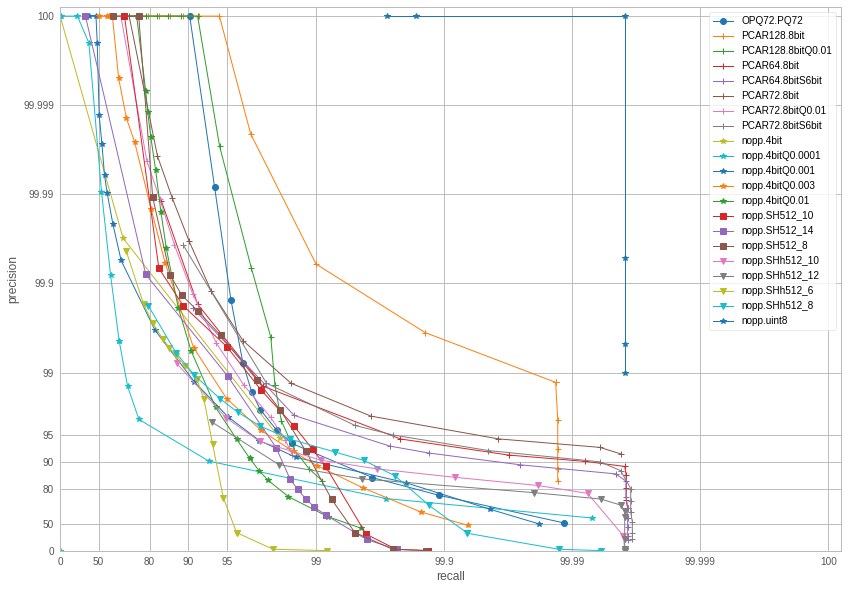
(Precision-recall. Note that the different codecs also have very different code sizes.)
The main variants are:
-
nopp.uint8 (144 bytes) is no encoding at all, which provides exact results — up to the recall without encoding.
-
PCAR128.8bit (128 bytes) is a scalar quantizer with a small dimensionality reduction to 128 dim. High accuracy but not much more compact than the original vectors.
-
nopp.SH512.xxx (512 bit = 64 bytes) are spectral hashing variants. SH512_10 (period 10) performs relatively well, but unfortunately below other options (it would have been a nice story to publish!)
-
OPQ72.PQ72 (72 bytes) is the traditional PQ used in Faiss. However it is outperformed by other codecs in terms of precision. PQ usually obtains the best accuracy in k-nn search but this does not extend to the range search in a high accuracy regime.
-
PCAR72.8bitS6bit (72 * 6 bits = 54 bytes) is a PCA to 72 dim followed by a 6-bit per component scalar quantizer (8bitS6bit = this is a simulated version). The other 4bit and 8bit variants are also scalar quantizers with various settings.
We chose the codec that offers precision > 90% and recall> 99.9% for the lowest memory usage: this is the 6-bit scalar quantizer with PCA to 72 dim: 54 bytes, 2.7x more compact than exhaustive storage.
This is the end of the small-scale experiments. We chose the partition and the codec, resulting in a setting that will hopefully scale to 1.5T vectors.
The result of this stage is an empty Faiss index with the proper preprocessing, quantizer, and codec, ready for use.
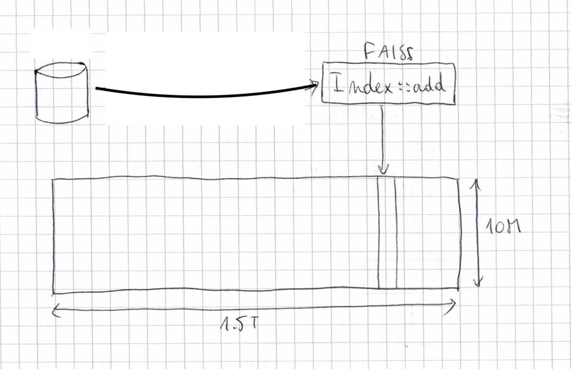
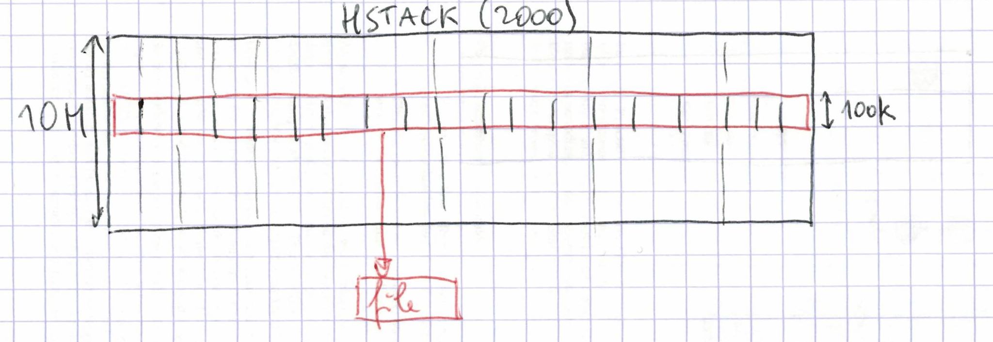
It is helpful to see the index of 1.5T vectors as a 10M-by-1.5T sparse matrix. Each vector in the index corresponds to one column with a single non-empty entry corresponding to the centroid that vector was assigned to. The entry contains the 54-byte code and a 8-byte id for the entry. Thus, the matrix will occupy 84TiB on disk. Of course, we use a large distributed file system to store this data. Note that in these experiments, we use relatively cheap spinning disk because we do not need fast random access to the data.
The storage of the matrix is in Compressed Sparse Row (CSR) format. This is equivalent to an inverted index, where each row corresponds to an inverted lists (aka posting list).
The difficulty is to split the indexing work into jobs that can be run in parallel on a cluster of machines, so that both the storage and processing are de-centralized.
The input data comes from a database that can be sharded into 2000 partitions of around 750M entries. We run 2000 cluster jobs to index the fractions. They just pull the data from the database and add the vectors to the empty index in RAM and store the result on disk. This takes around 7.5h per fraction on a cluster machine. Each of the 2000 indexes can be seen as a slice of columns in the big matrix.
At this point we are moving to an on-disk representation (OnDiskInvertedLists). This means that the data of an index is stored on disk, and memory mapped. This makes it possible to have indexes larger than RAM, at the cost of slower accesses. Also, the limiting factor of all operations is read and write speed on disk. To set expectations: for sequential reads on a quiet day, our distributed FS can sustain 200-700 MiB / s from a single host.
Faiss now has a functionality where OnDiskInvertedList's can be concatenated into a big index (as in numpy.hstack), so the 2000 indexes can already be used as a single index. However:
- the metatdata of 2000 indexes (begin and end pointer of each list) is too large to fit in a server with 256G RAM!
- even if it would fit, the search would be horribly slow because scanning a single row of the matrix would require 2000 disk seeks.
Therefore, the data needs to be re-organized.
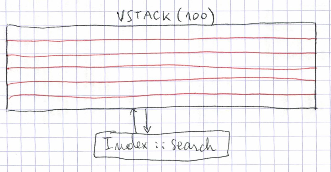
The data should be split over inverted lists, so that scanning a row of the matrix corresponds to a linear scan on disk. For this, we split the matrix into 100 files of 100k inverted lists each, each generated by a cluster job. We can do this in a single machine without running out of RAM by loading only the meta-data for 100k lists at a time for the 2000 column splits.
The data is read sequentially from 2000 files and written sequentially to one output file per row slice.
Each of the 100 jobs runs in between 24 and 33 h. This is quite slow: 930 GB in 24 h = 10 MB/s. This inefficiency may be due to the fact that all 100 jobs are reading from the same 2000 files.
The 100 row splits can be combined with a hstack into an index that can be searched in Faiss.
This shows up as an impressive 83TiB memory map in top on the machine we run it on:
 PID     USER     PR NI  VIRT    RES    SHR S  %CPU %MEM    TIME+ COMMAND
 2118311 matthijs 20  0 83.6t 142.8g 136.6g D 155.0 56.8 54:06.76 python3.6
This just works from a python notebook on a modest server, no need for special server daemons because the distribution is taken care of by the distributed FS.
At this stage, the search performance of this index is quite low. A single query can take up to a few minutes. So now we have to improve that performance.
Let's read a few hundred random rows from the matrix from several threads. For example for 16 threads this can be visualized as:
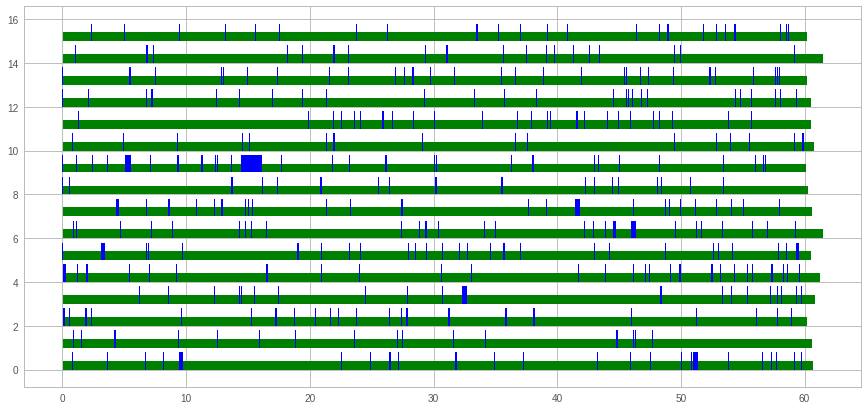
The x-axis is time (seconds) and the y-axis is what each thread is busy with. In blue is the time spent waiting for the first byte to arrive, and in green is the subsequent time spent to read the whole inverted list. Since there is more green than blue, it is obvious that throughput is more important than latency (seek time). We also observed that to read a fixed number of inverted lists, 32 threads are optimal.
Each search retrieves nprobe inverted lists and scans them to compute distances. Each distance computation requires to read 54 bytes. Thus, the number of distances and amount of memory scanned is not uniform across queries. To investigate search time in real cases, we look at the search time as a function of the number of computed distances, over a few hundred queries at nprobe=64. This gives:
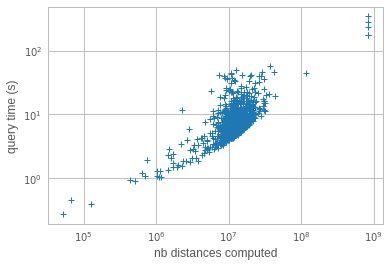
o it turns out that there are a few queries that are very slow. They scan almost 1B elements sequentially! In fact, reading 1B elements, or 54GB of data, in 120 s is actually quite efficient (500 MiB/s from disk). Why are they reading so much data? It turns out that the inverted lists sizes are unbalanced. The list lengths, sorted by size look like:
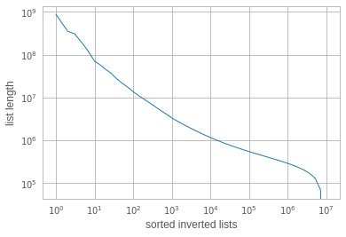
ie. there are <10 lists that have more than 100M elements, when the average list length is 150k! However, how comes that these lists appear in 4 out of a few hundred queries? If list sampling was uniform, they should not be hit so often?
This is a well known effect in inverted files: the longest inverted lists are also the ones that are most likely to be accessed. Since the inverted list sizes reflect the data distribution, an imbalance in the list sizes has a quadratic effect on search time.
To work around the performance issue, we de-duplicated the 30 largest inverted lists. In addition to some tweaking of the threading, and a proper warm-up of the memory maps, this brings down the average search time to ~2s for nprobe=64 or ~20s for nprobe=512.
This is a data transfer rate of 250-300 MiB / s, which is already high, so it is unlikely we can do much better on a single machine. However, it would be nice it we could be a little faster than that, because in reality we will use it at nprobe=512.
Since the limiting factor is data access, the obvious workaround is to distribute the search over several machines and recombine the results. Thus, we implemented a client-server version of the search, and started up 20 servers. The master and the 20 slaves operate on exactly the same index.
At query time, the master finds the 512 lists to scan. Then it instructs the 20 slaves to scan each a subset of the lists. The load is balanced so that each server has approximately the same amount of data to load. They then send back the the results to the main machine.
This results in a search speed of 2 to 6s per query for nprobe=512. When batching the searches and setting nprobe=64, this can be reduced to 1s per query.
This study is a proof-of-concept for the index. It showed that vanilla Faiss with an on-disk file-based storage can be used with interactive performance.
The code for these experiments can be found here: Distributed on-disk index. It runs at scale 1/1000th on the Deep1B dataset.