Indexing 1G vectors
For those datasets, compression becomes mandatory (we are talking here about 10M-1G per server). The main compression method used in Faiss is PQ (product quantizer) compression, with a pre-selection based on a coarse quantizer (see previous section). When larger codes can be used a scalar quantizer or re-ranking are more efficient. All methods are reported with their index_factory string.
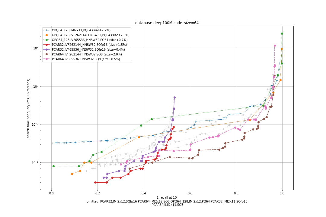
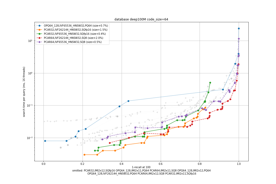
In the tests below we use the the Deep1B (96-dim activations from a neural net) and Bigann (128-dim SIFT descriptors) datasets. Both datasets have 1B database vectors and 10k queries. For smaller databases we use the N first database vectors. We report the 1-recall@1 measure that is most sensitive. For illustration, we also report the 1-recall@100 for a single setting: Deep100M with 64-byte codes.
We report only the IVFx_HNSW and IVFx(IVFy,PQfs,RFlat) variants for the coarse quantizer.
IMI is usually less efficient in terms of speed-precision tradeoff.
Larger values of the number of centroids have a slightly higher asymptotic accuracy, but the index is also slower to build.
Click on the triangles to see the speed vs. precision tradeoffs plots for a fixed code size.
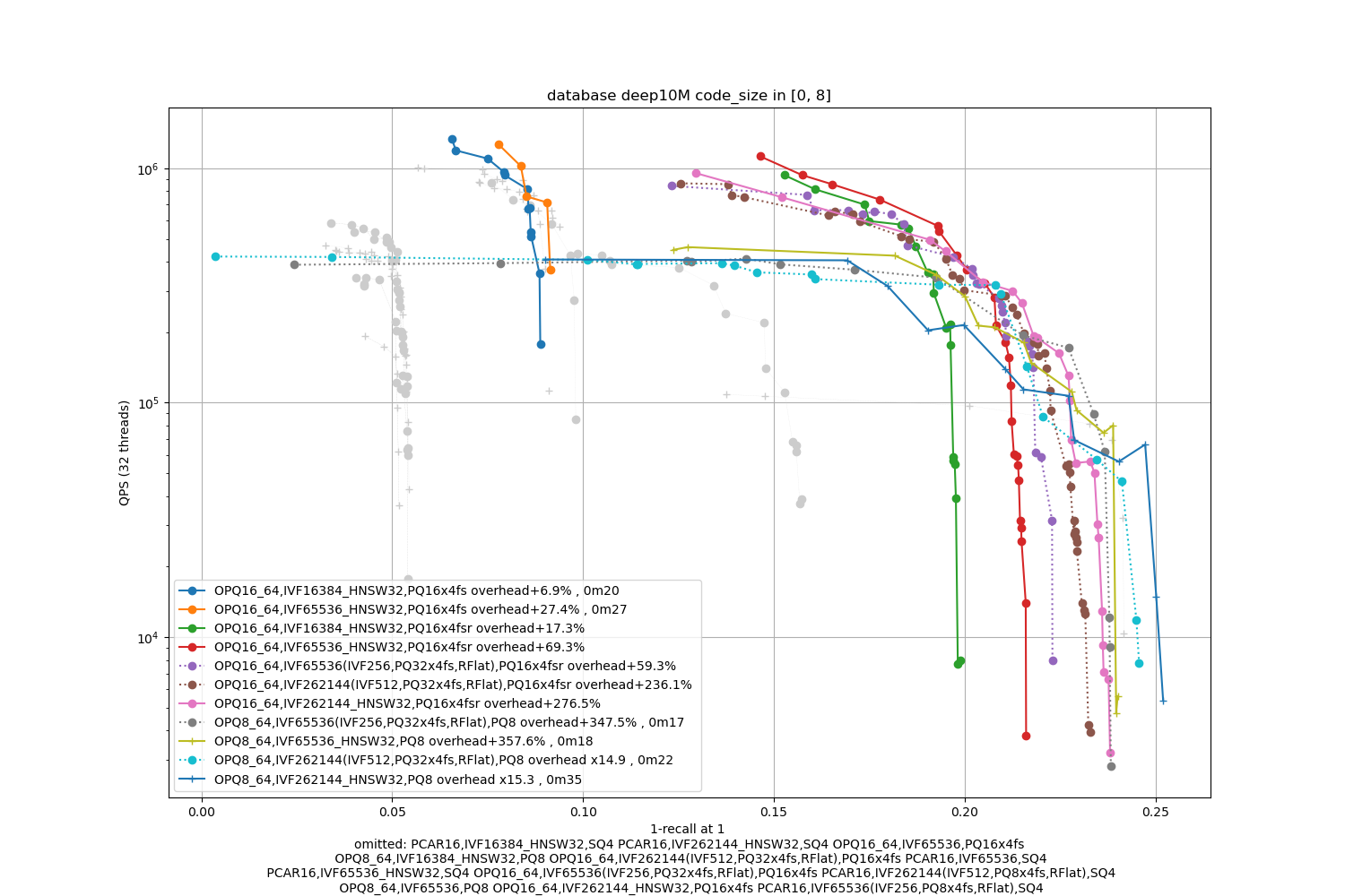
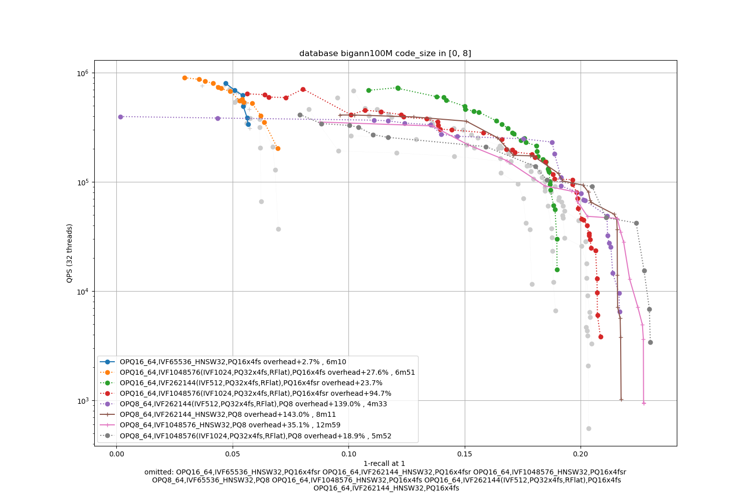
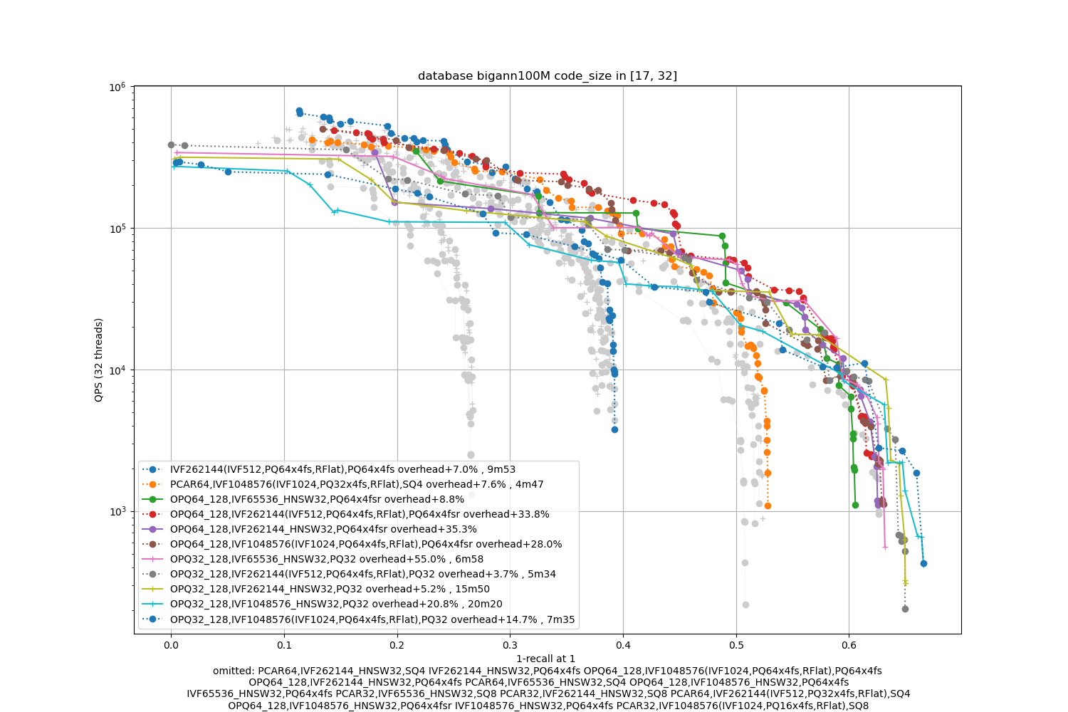
For all benchmarks we report plots of an accuracy measure (x-axis) vs. the number of queries per second (QPS, y-axis): up and right is better. All experiments were performed on a normalized platform (2.2 GHz Xeon E5-2698, 80 cores). We did perform all experiments with 32 cores. This is to simulate an environment with a diverse set of tasks with some memory stress (in 1-thread mode the computational load is unrealistically important compared to memory access time). The plots report only the combinations that are optimal for at least one operating point, others are in light gray.
All experiments were performed with the code in bench_all_ivf.
For each of the dataset sizes, we also report the exact runtime parameters used to get the result. They appear in the format:
parameters                                   R@1   R@10  R@100  time(ms/q)   nb distances #runs
...
nprobe=64,quantizer_efSearch=32          0.6421 0.8104 0.8123      0.03028       72094677    10
nprobe=128,quantizer_efSearch=32         0.6786 0.8680 0.8700      0.05387      142670158    6
...
This means that by setting the parameters nprobe=128,quantizer_efSearch=32 with the ParameterSpace object, we obtain 0.6786 recall@1 for that dataset, the search will take 0.05387 ms per query.
The total number of distances computed for the 10k queries is 142670158 and this measurement was obtained in 6 runs (to reduce jitter in time measurements).
Any efficient index for k-nearest neighbor search can be used as a coarse quantizer.
In the follwing we compare a IVFPQFastScan coarse quantizer with a HNSW coarse quantizer for several centroids and numbers of neighbors k, on the centroids obtained for the Deep1B vectors.
We report the best QPS where the intersection measure is >= 99% because
a coarse quantizer usually runs in a high precision regime, especially at add time (no multiple assignment).
details
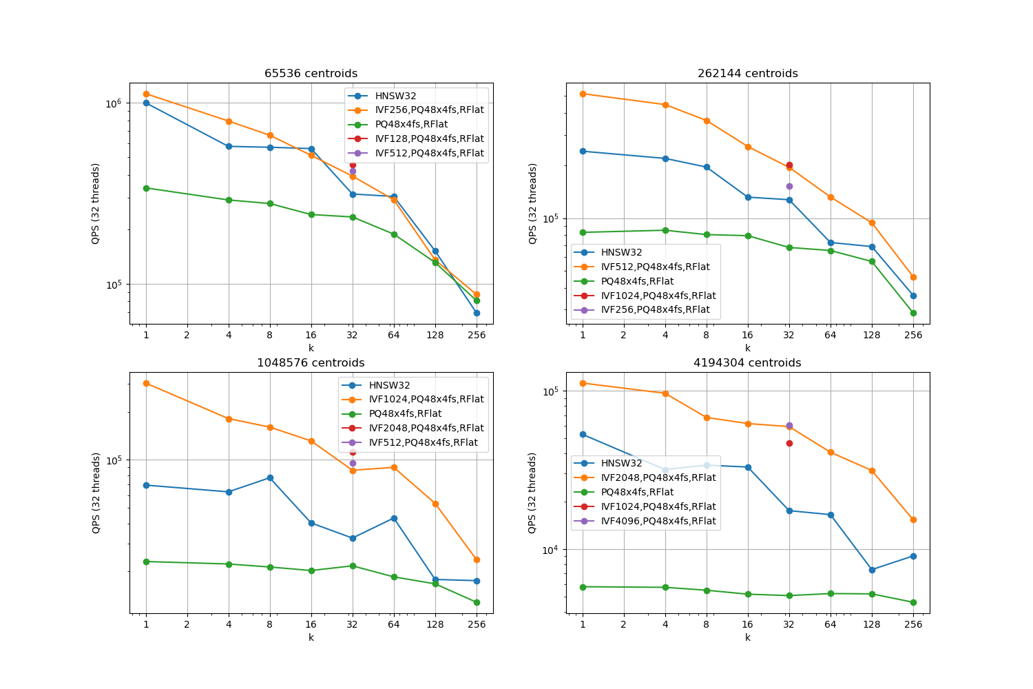
Observations:
-
the k=1 setting is critical because it is used at add time for the IVF.
-
IVFPQFastScan is competitive with HNSW for most operating points, but it is harder to tune because it depends on two parameters (nprobe and k_factor) instead of one (efSearch).
-
for 65536 centroids, the difference between HNSW and IVFPQFastScan is not very significant.
-
getting an intersection >= 99% for k=1 requires setting nprobe=32 and k_factor=32. It is critical to set this before adding elements to the index.
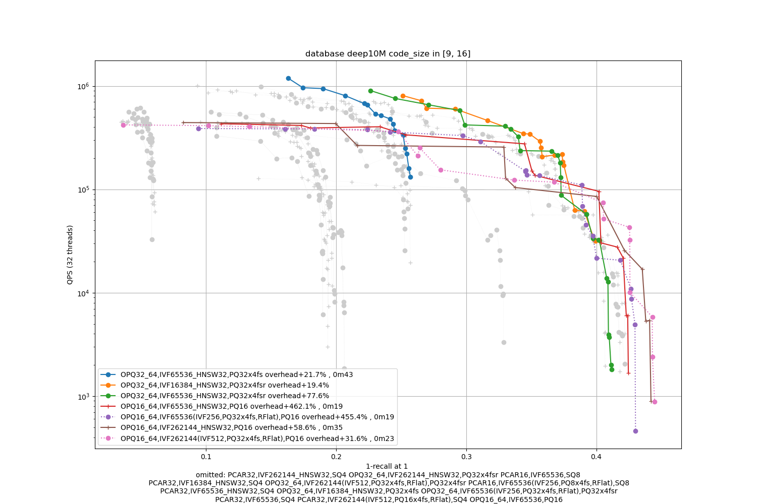
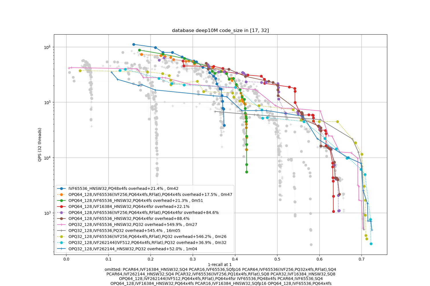
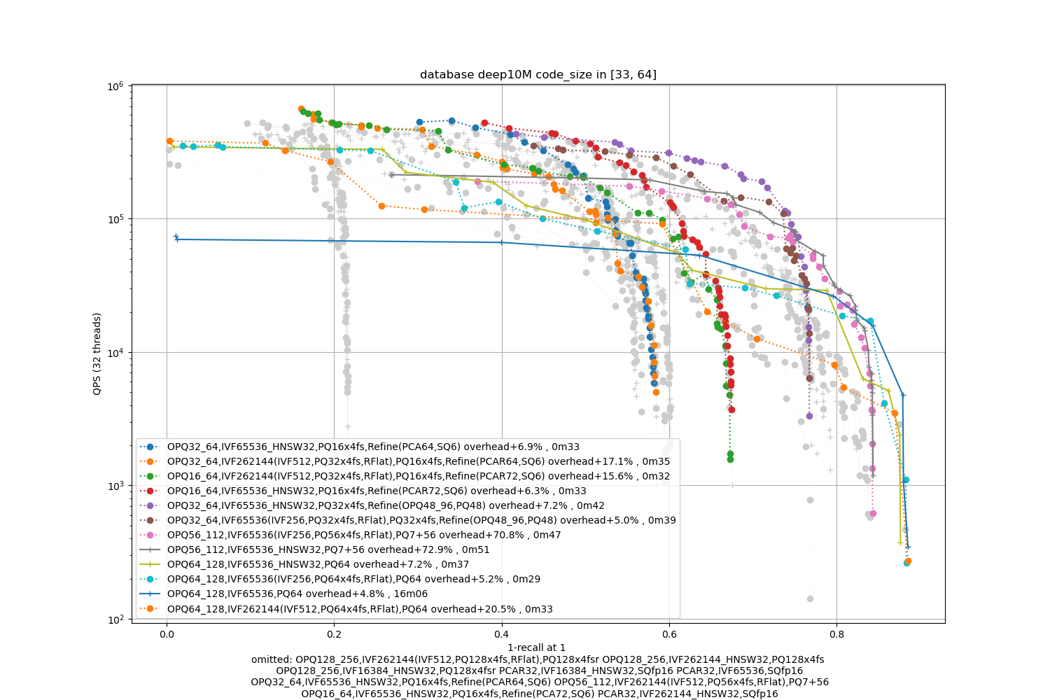
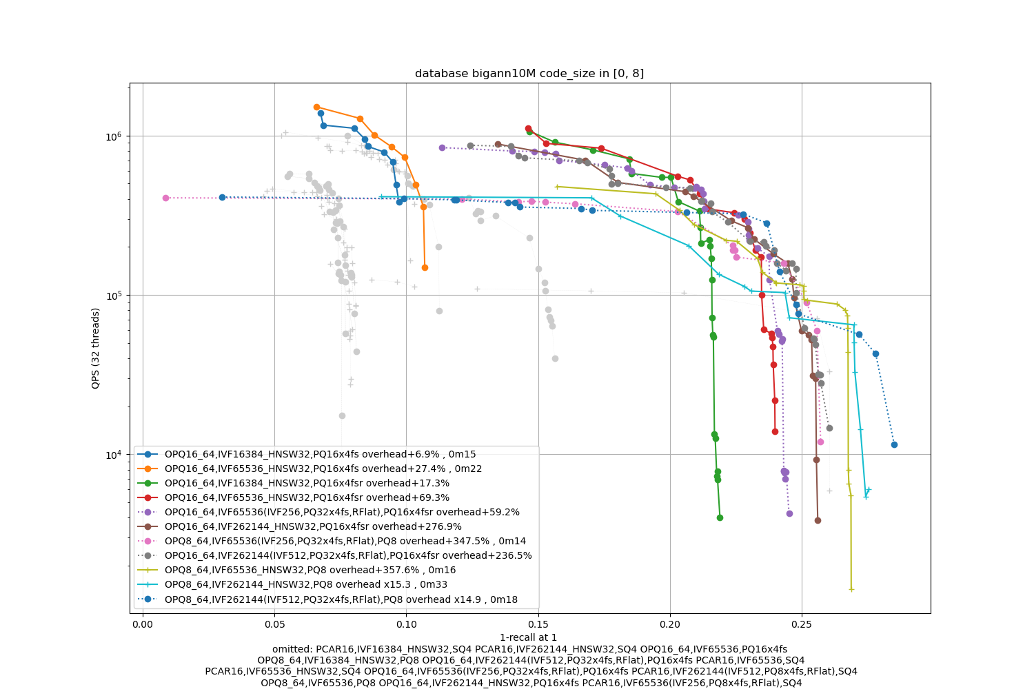
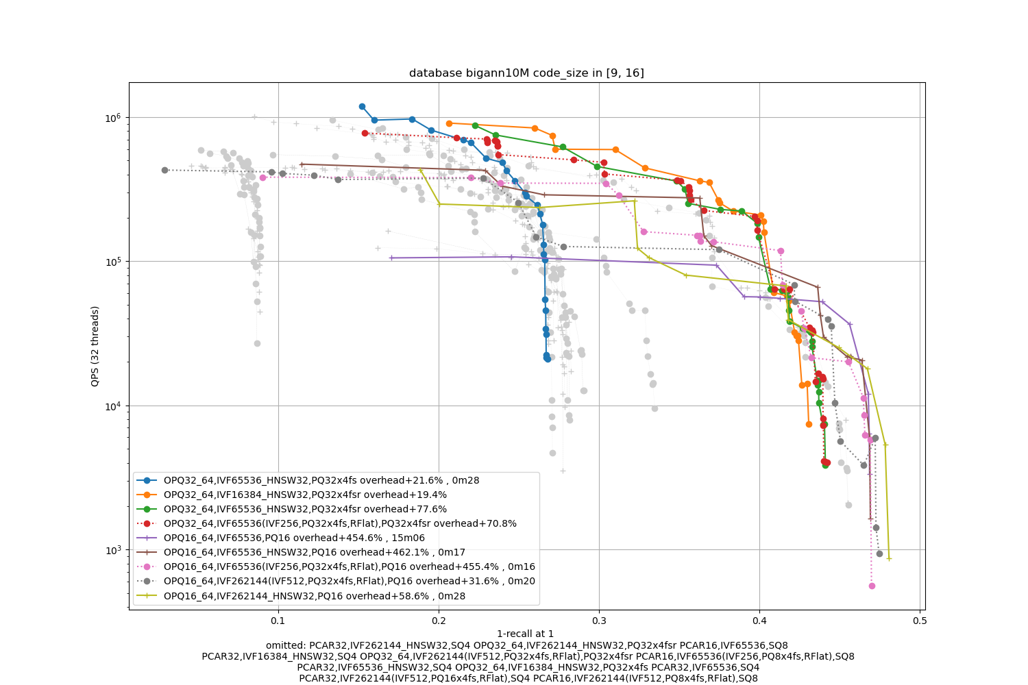
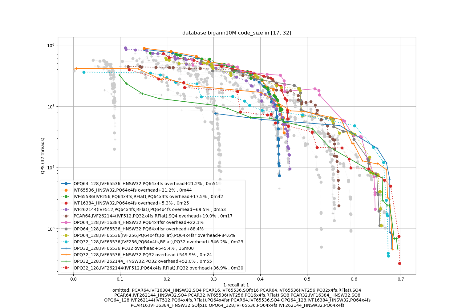
Results are broken down per code size (8, 16, 32, 64 bytes per vector). We test:
-
the most promising coarse quantizers (sizes 16k, 65k and 262k) with HNSW and IVFPQFastScan ANN structures
-
PQ, PQfs, SQ encodings of the relevant sizes with PCA or OPQ preprocessing
-
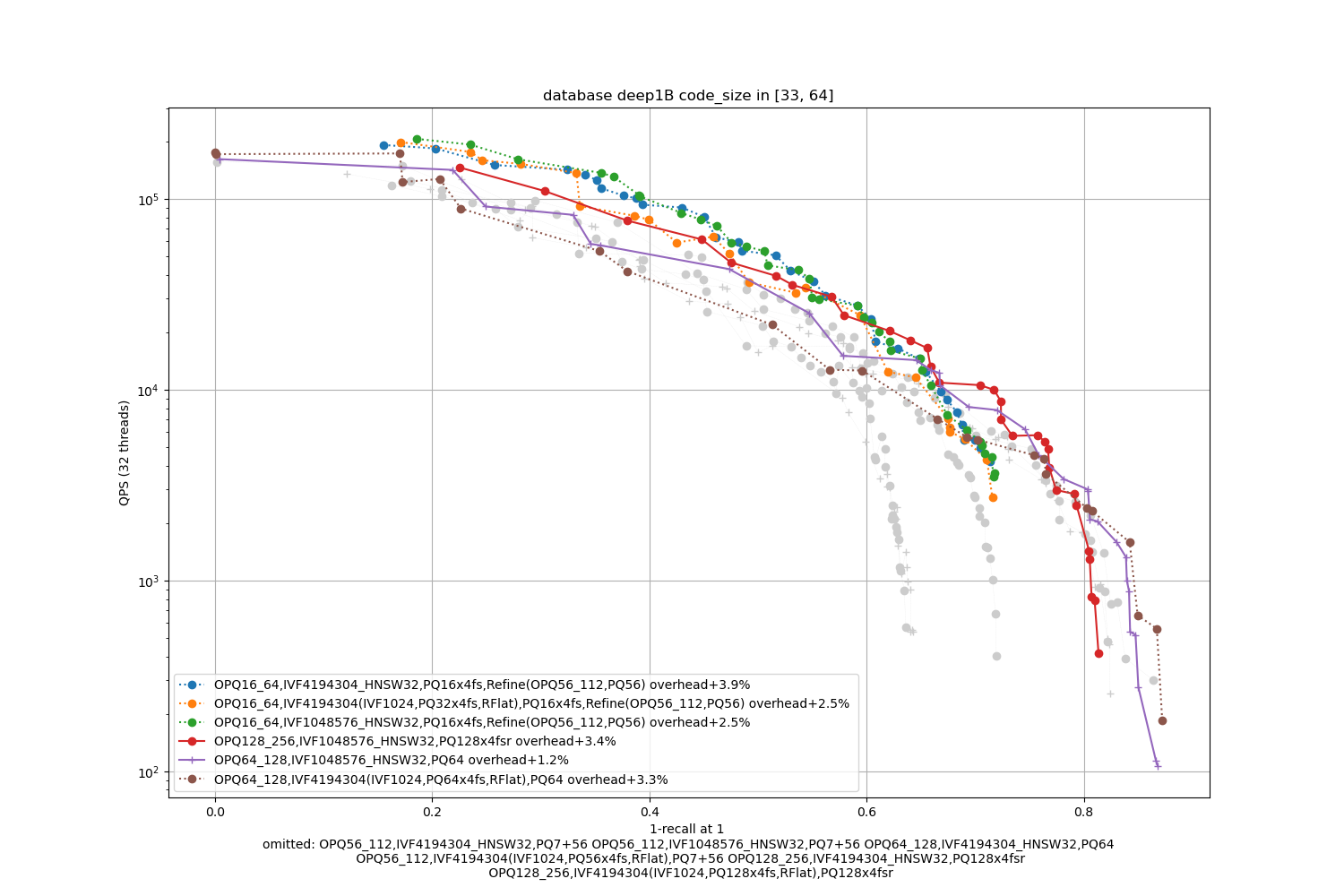
for code size 64, we also test PQfs re-ranking options with either a Refine index or with an IndexIVFPQR (PQ7+56) that in addition uses a residual encoding.
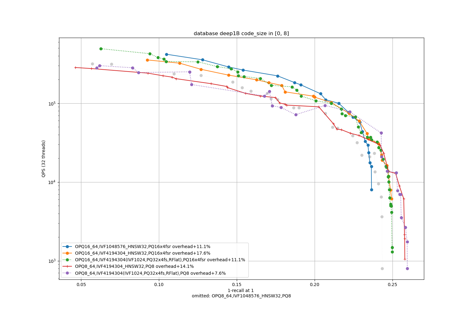
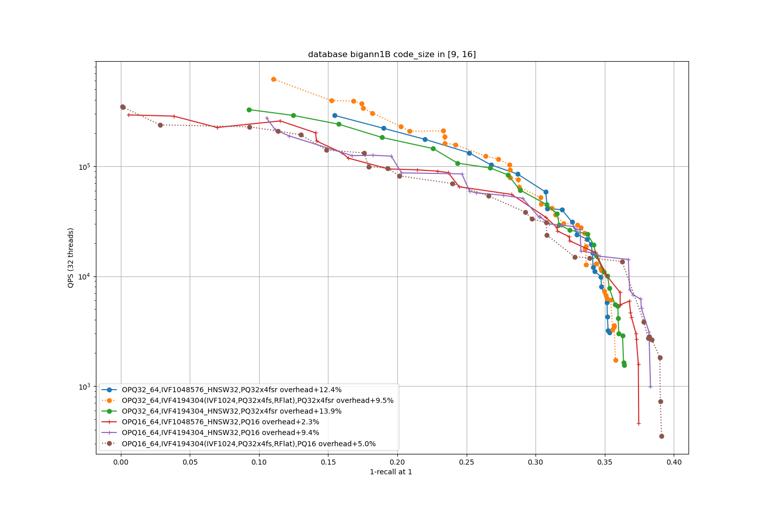
In terms of codes:
- the best topline precision is always obtained with a PQ as encoding
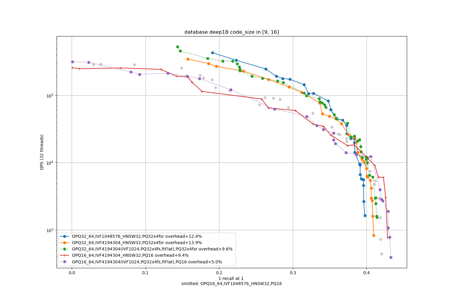
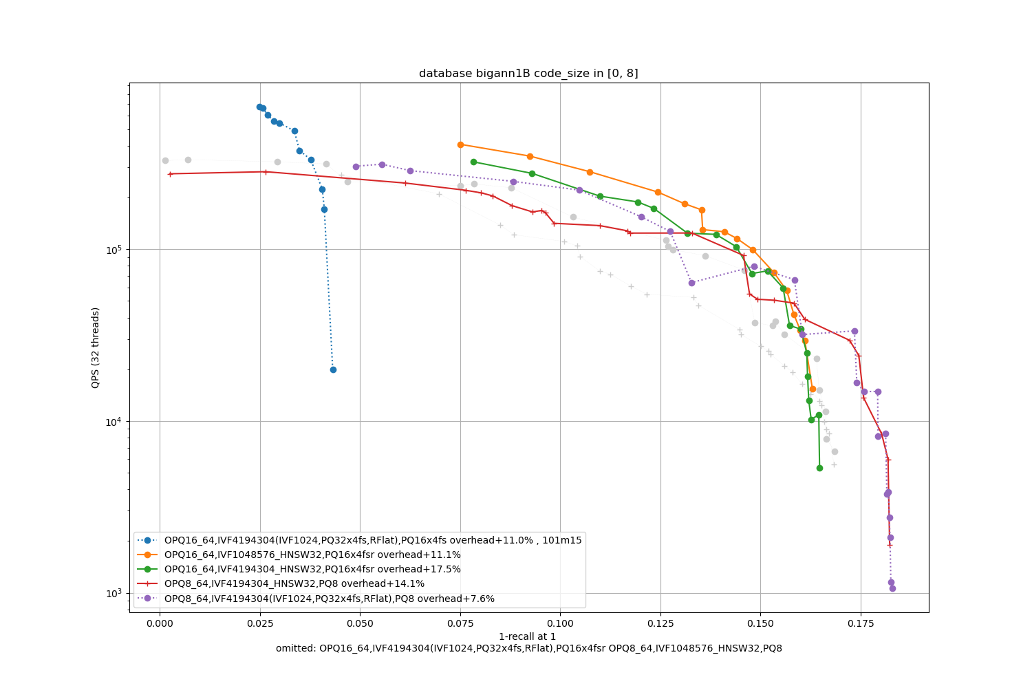
- for faster / less accurate operating points the PQ 4-bit fast scan variants (PQx4fsr) are a good choice because they are well optimized, they outperform the SQ on almost all operating points (but are slower to index).
- the gap narrows down for longer codes (32 and 64 bytes per code)
- for recalls at ranks > 1 the difference is not so important. It mainly matters for 1-recall@1 performance (the one that is reported)
The memory (RAM) usage consists of:
- the codes
- the ids corresponding to codes (8 bytes per item)
- the quantizer's size, inverted list pointers + length (at least 16 bytes per centroid), pecomputed tabels for PQ -- note that the new default for Faiss is to not compute tables if the tables are above 2GB in size (an arbitrary number that may be too big for small indexes or could be higher for bigger indexes). The overheads are reported in the caption as + a certain %.
- invisible overheads: vector geometric reallocation buffer, etc. These are not reported because they are difficult to measure.
Deep10M, 8 bytes / code
Deep10M, 16 bytes / code
Deep10M, 32 bytes / code
Deep10M, 64 bytes / code
bigann10M, 8 bytes / code
bigann10M, 16 bytes / code
bigann10M, 32 bytes / code
bigann10M, 64 bytes / code

Detailed logs with runtime parameters: Deep10M bigann10M
As a coarse quantizer, we tried 65k, 262k and 1M centroids, indexed with either HNSW or a IVF with refinement.
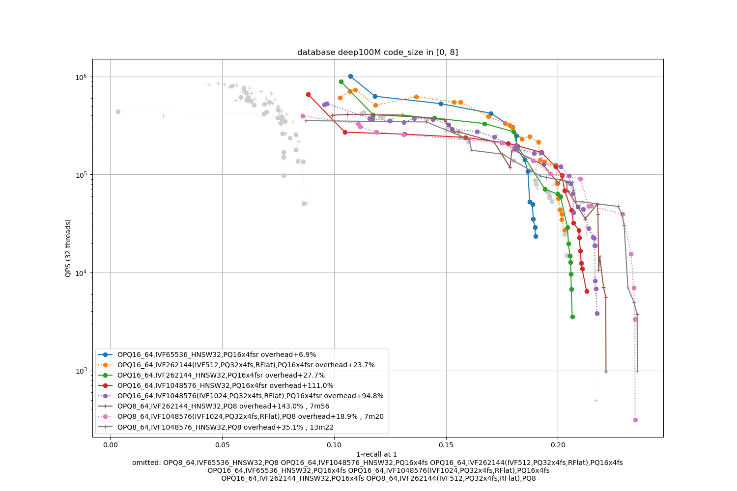
Deep100M, 8 bytes / code
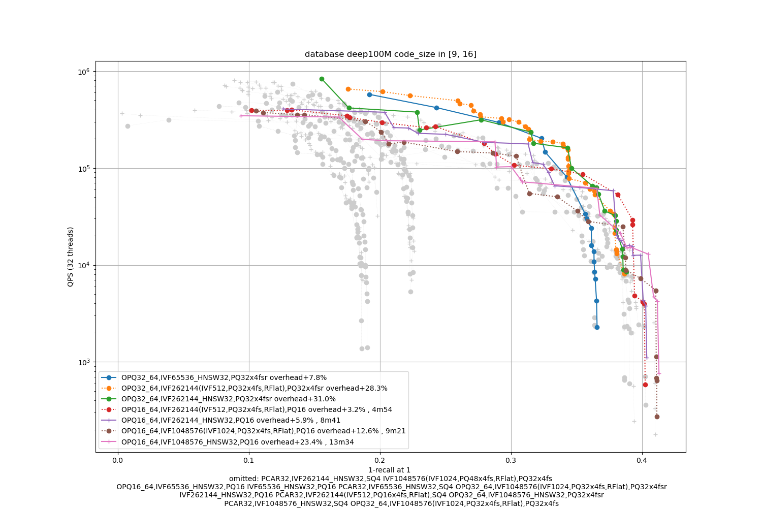
Deep100M, 16 bytes / code
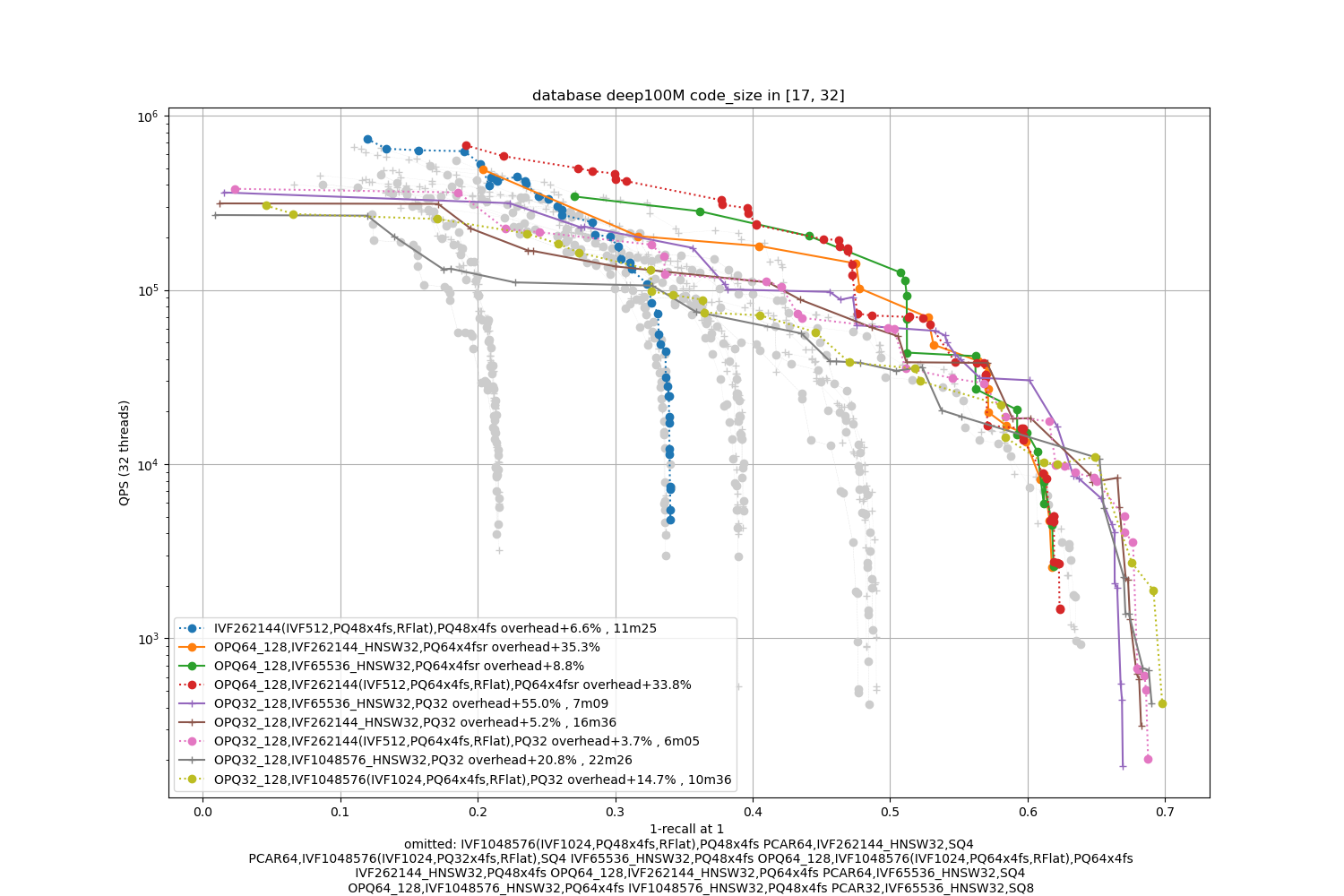
Deep100M, 32 bytes / code
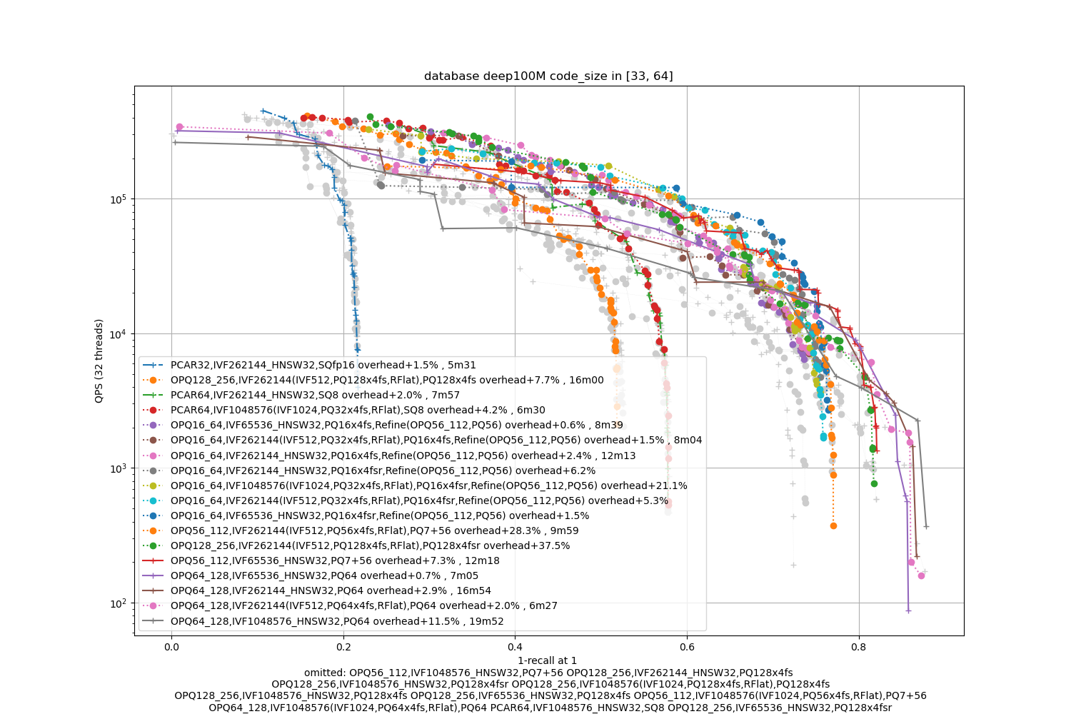
Deep100M, 64 bytes / code
bigann100M, 8 bytes / code
bigann100M, 16 bytes / code

bigann100M, 32 bytes / code
bigann100M, 64 bytes / code

Detailed logs with runtime parameters: Deep100M bigann100M
The datasets are 10x bigger. We also indicate the index building time (with 24 threads, excluding the training time).
Observations:
-
the advantage of IVF with 4-bit PQ compared to HSNW as a coarse quantizer is not obvious. Therefore, HSNW is attractive because it has fewer parameters to train.
-
the fsr variants are the best in the average accuracy regime
Note that for 1M and 4M centroids we trained the vocabulary on GPU before building the index, otherwise k-means is very slow. All other operations are on CPU.
Deep1B, 8 bytes / code
Deep1B, 16 bytes / code
Deep1B, 32 bytes / code

Deep1B, 64 bytes / code
bigann1B, 8 bytes / code
bigann1B, 16 bytes / code
bigann1B, 32 bytes / code
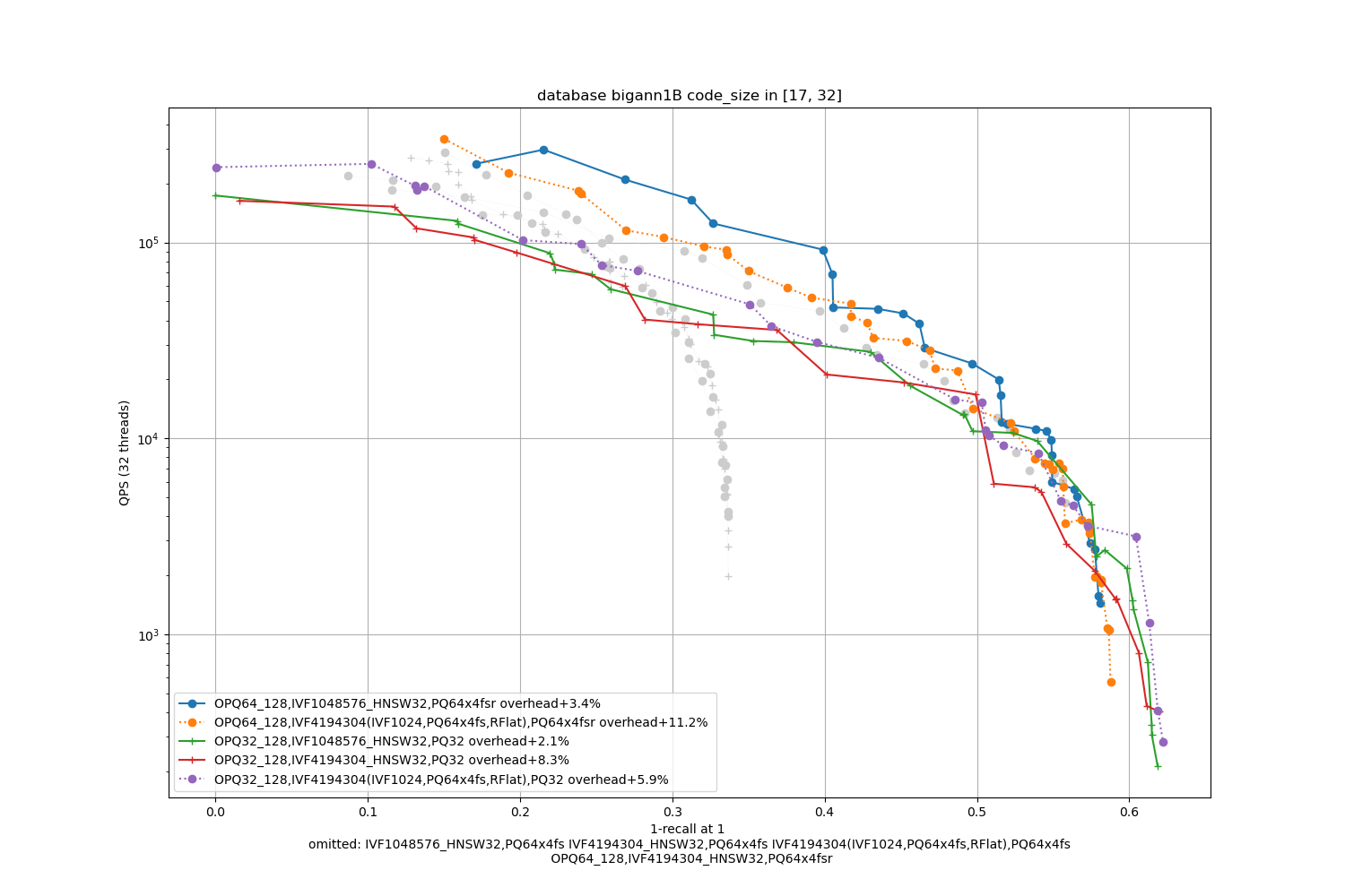
bigann1B, 64 bytes / code

Detailed logs with runtime parameters: Deep1B bigann1B
Also includes some GPU comparisons.
archived
The Bigann dataset is a classical benchmark used in computer vision. It contains 1 billion SIFT descriptors. The plot below shows that it is relatively easy to index:
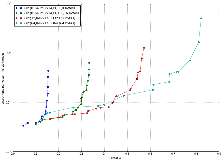
These results were obtained with bench_polysemous_1bn.py:
python bench_polysemous_1bn.py SIFT1000M OPQ8_64,IMI2x14,PQ8 autotuneMT
Another research dataset that was introduced in this CVPR'16 paper. It contains 1Bn 96D descriptors.
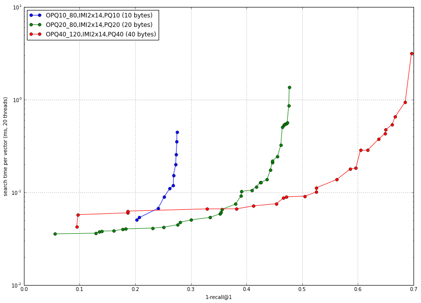
A recent CVPR'16 paper has a GPU implementation for the search. We experiment with relatively low-precision operating points (8 bytes per code) to allow for a direct comparison with published papers. Note however that for high quality neighbors, more bytes would be required (see above).
| Method | Hardware | R@10 | query time (ms) / vector |
|---|---|---|---|
| Wieschollek et al. CVPR'16 | Titan X | 0.35 | 0.15 |
| OPQ8_64,IMI2x13,PQ8x8 | CPU (1 thread) | 0.349 | 0.4852 |
| " | CPU (20 threads) | 0.349 | 0.035 |
| OPQ8_32,IVF262144,PQ8 | Titan X | 0.376 | 0.0340 |
| " | " | 0.448 | 0.1214 |
(methods are described with their index_factory string)
The operating point we are interested in is one that takes ~25 GB of RAM, which corresponds to 20-byte PQ codes. The first row is the best operating point we are aware of at the time we made the comparison. The other rows correspond to different operating points achieved by CPU- and GPU-Faiss algorithms.
| Method | Hardware | R@1 | query time (ms) / vector |
|---|---|---|---|
| Babenko & al. CVPR'16 | CPU (1 thread) | 0.45 | 20 |
| OPQ20_80,IMI2x14,PQ20 | CPU (1 thread) | 0.4561 | 3.66 |
| OPQ20_80,IVF262144,PQ20 | 4*K40 | 0.488 | 0.18 |
| " | 4*K40 | 0.493 | 1.1 |
| OPQ32,IVF262144,PQ32 | 8*TitanX | 0.671 | 0.2328 |
| OPQ64_128,IVF262144,PQ64 (float16 mode) | 8*TitanX | 0.856 | 0. 3207 |