Segment individual trees and compute metrics
Document updated on February 13th 2020 and up-to-date with
lidR v3.0.0
The following example shows how to process your file entirely in the R environment using the lidR package. The file used in this work can be downloaded here. This work is the "lidR version" of the blog article published on quantitative ecology.org. We will use the same file to do (almost) the same things but using fewer lines of code.
First we need to read the file. For this we only need the spatial coordinates. ScanAngle, Intensity and so on are not useful. While Classification of the points is important for computing the digital terrain model, this task was not already done so we must perform that task ourselves.
library(lidR)

las = readLAS("Example.las")
plot(las)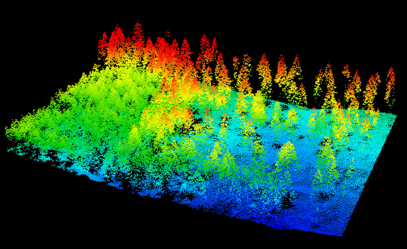
classify_ground provides a several algorithm to classify ground points. This function is convenient for small-to-medium plots like the one we are processing but I do not recommend it for large catalog of file files. Here we use the csf algorithm because it works well without need to tune the parameters.
las = classify_ground(las, csf())
plot(las, color = "Classification")We need to set the ground at 0. We could subtract the DTM to obtain ground points at 0 but here we won't use a DTM but we will rather interpolate each point exactly.
It is important to notice here that neither the ground classification nor the DTM interpolation where performed using a buffer around the region of interest. Thus we can expect a poor height normalization at the egdes of the dataset. But we will consider that fair enough for the purpose of this tutorial.
las = normalize_height(las, tin())
plot(las)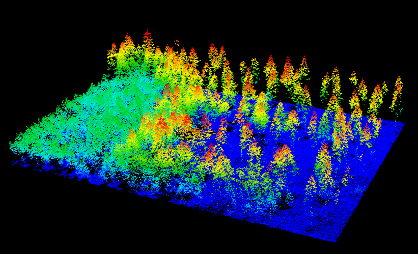
There are several methods to segment the tree in lidR the following will use a watershed, that is far to be the best, but is good enough for this easy to segment example.
In the next steps we will use an algorithm that requires an canopy height model. This step can be skipped if you chose an algorithm that performed the segmentation at the point cloud level. So, let's compute a digital surface model with the pit-free algorithm (see also canopy height models in lidR).
algo = pitfree(thresholds = c(0,10,20,30,40,50), subcircle = 0.2)
chm  = grid_canopy(las, 0.5, algo)
plot(chm, col = height.colors(50))
Optionally we can smooth this CHM using the raster package
# smoothing post-process (e.g. two pass, 3x3 median convolution)
ker = matrix(1,3,3)
chm = focal(chm, w = ker, fun = median)
chm = focal(chm, w = ker, fun = median)

plot(chm, col = height.colors(50)) # check the image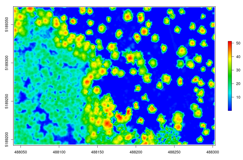
The segmentation can be achieved with segment_trees. Here I chose the watershed algorithm with a threshold of 4 meters. The point cloud has been updated and each point now has a number that refers to an individual tree (treeID). Points that not trees are assigned the id value NA.
algo = watershed(chm, th = 4)
las  = segment_trees(las, algo)

# remove points that are not assigned to a tree
trees = filter_poi(las, !is.na(treeID))

plot(trees, color = "treeID", colorPalette = pastel.colors(100))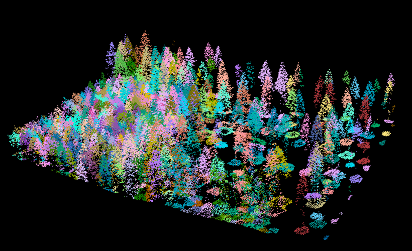
hulls  = delineate_crowns(las, func = .stdmetrics)
spplot(hulls, "Z")
In the previous example, even if the segmentation is done using a canopy height model, the classification has been made on the point cloud. This is because lidR is a point cloud oriented library. But one may want to get the raster to work with rasters. In that case the function watershed can be used standalone:
crowns = watershed(chm, th = 4)()
plot(crowns, col = pastel.colors(100))
Once you are working with rasters the lidR package is not implied anymore. User can rely on the raster package for further analysis. For example:
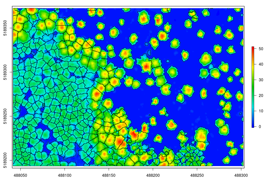
contour = rasterToPolygons(crowns, dissolve = TRUE)

plot(chm, col = height.colors(50))
plot(contour, add = T)