Make cheap High Performance Computing to process large datasets
Document updated on September 19th 2019 and up-to-date with lidR v2.2.0
When testing long and complex new algorithms that need to be tested and debugged on large datasets (e.g. above 1000 km²) we can face a problem of computation time. When running a function only once, we can wait for the output. But when we have to run the function again and again and again the computation time becomes a problem. We don't want to wait a full night to know if the function does work as expected... and another night to know if our bug fix works...
Hopefully the lidR package has been designed, from the beginning (but never tested until v2.1.3) to work on multiple machines.
In this tutorial we will build a cheap multi-machine HPC using our colleagues computers.
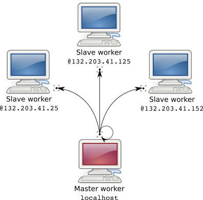
In my team we have several computers. There is my computer and my old computer with a broken screen (screens are useless to compute remotely). There are also Bob's and Alice's computers. Bob and Alice mainly write text and thus do not use intensively their computers. So I used their unexploited power to spread my computations on 4 machines.
Because we are all connected under the same local network it is extremely easy to access a machine remotely as long as the machine is a ssh server. This enables me to complete 6 hours computations in 1h30 transparently as if it was computed on my own machine.
Note: this works either on Windows, GNU/Linux or MacOS however the configuration on GNU/Linux takes a few minutes while doing the same on Windows is more complex. So I'll describe the GNU/Linux set-up and provide links for other OSes.
To access a machine remotely it must be a ssh server. So, we need to install a ssh server on each machine. For Windows I suggest this page to start.
sudo apt-get install ssh
Now to access each machine remotely we need their local IP address. For Windows I suggest this page.
hostname -I
Then try to connect to the machines remotely from the master machine to see if it works.
ssh bob@132.203.41.125
If you are able to connect to the machines remotely your are almost done. At this stage you can use a public RSA key to log automatically in each computer (see this page). This is not mandatory but very convenient.
On real HPC, each machine can access data using a massively parallel file sharing system. On our cheap HPC each remote worker could, in theory, access the data from the master worker but the transfer will pass through the local network and is likely to represent gigabytes of traffic. So in practice it is not workable. So instead we will copy the dataset on each machine. Each machine will access the data from its own drive. Once each machine has a copy of the dataset we are done. We can use remote futures:
library(lidR)
library(future)

plan(remote, workers = c("localhost", "jr@132.203.41.25", "bob@132.203.41.152", "alice@132.203.41.125"))

ctg = readLAScatalog("~/folder/LASfiles/")
metrics = grid_metrics(ctg, .stdmetrics, 20)
And we are done!! We are computing on 4 different machines!
Well... almost... This is true only if all the files are stored within the same path on each computer which is unlikely to be the case. For example on Alice's machine data are stored in /home/Alice/data/ but on Bob's machine they are in /home/Bob/remote/project1/data/. So we need a tweak to propagate this information. But first we need to understand how it works.
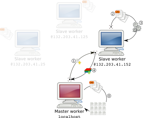
When processing a LAScatalog in parallel, either locally or remotely, the catalog is first split into chunks in the master worker (step 0 in figure 2). Then, each worker processes a chunk, when it is done it processes another chunk and so on until each chunk is done.
A chunk is not a subset of the points cloud. What is sent to each worker instead is a tiny internal object named LAScluster that roughly contains only the bounding box of the region of interest and the files that need to be read to load the according points cloud (step 1 in figure 2).
Consequently the bandwidth needed to send a workload to each worker is virtually null. This is also why the documentation of catalog_apply() mentions that each user-defined function should start with readLAS(). Indeed each worker reads its own data (step 2,3 in figure 2).
Once a worker is done with one chunk the output is returned to the master worker (step 4 in figure 2). At this stage, depending on the size of the output it might be demanding for the network. grid_*() functions return Raster* objects so it is not a big deal. However, running las* functions that return LAS objects might not be suitable. In this case we can use opt_output_file() and each worker will write its own data locally. What is returned is the latter case is the path to the data i.e. a virtually 0 bytes object.
In our cheap HPC, each worker reads its own files with a specific path which is unknown by the master worker when building the lightweight chunks (LASclusters). The master worker only knows the path of the files read with readLAScatalog(). In version lidR v2.2.0 there is an undocumented features to provide alternative directories.
ctg = readLAScatalog("~/folder/LASfiles/")
ctg@input_options$alt_dir = c("/home/Alice/data/", "/home/Bob/remote/project1/data/")
This is it! We have made a functional cheap HPC!
library(lidR)
library(future)
plan(remote, workers = c("localhost", "jr@132.203.41.25", "bob@132.203.41.152", "alice@132.203.41.125"))
ctg = readLAScatalog("~/folder/LASfiles/")
ctg@input_options$alt_dir = c("/home/Alice/data/", "/home/Bob/remote/project1/data/")
metrics = grid_metrics(ctg, .stdmetrics, 20)
For older versions of lidR the tweak is more complex to achieve... just update to v2.2.0.