Area based approach from A to Z
Document created on July 26th 2019 by @ptompalski and @tgoodbody, updated on February 13th 2020 and up-to-date with lidR v3.0.0
This page demonstrates how to process ALS point cloud data to create wall-to-wall predictions of selected forest stand attributes using an area-based approach (ABA) to forest inventories. The steps used in this vignette as well as further details about enhanced forest inventories (EFI) are described in depth in White et al. 2013 and White et al. 2017.
This vignette assumes that the user has a directory of classified and normalized ALS tiles.
library(lidR)
library(sf)The function readLAScatalog builds a LAScatalog object from a folder. LAScatalog objects produce regions of interest (ROIs) from each ALS file within the catalog directory. Make sure the ALS files have associated index files - for details see: Speed-up the computations on a LAScatalog.
ctg <- readLAScatalog("path/to/ALS/data")
print(ctg) # See details of the catalog object

#> class       : LAScatalog
#> extent      : 297317.5 , 316001 , 5089000 , 5099000 (xmin, xmax, ymin, ymax)
#> coord. ref. : +proj=utm +zone=18 +ellps=GRS80 +towgs84=0,0,0,0,0,0,0 +units=m +no_defs
#> area        : 125.19 km²
#> points      : 1.58 billion points
#> density     : 12.6 points/m²
#> num. files  : 138
To visualize the ROIs use the plot function on your LAScatalog object.
plot(ctg)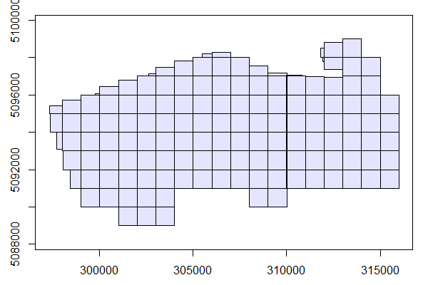
Now that our ALS data is prepared lets read in our inventory data using the st_read function from the sf package. We read in a .shp file where each features is a point with a unique plot ID and corresponding plot level inventory summaries. Our plots object contains 203 plots with coordinates of plot centers, plot name, and stand attributes: Lorey's height (HL), Basal area (BA), and gross timber volume (GTV).
plots <- st_read("PRF_plots.shp")
plots

#> Simple feature collection with 203 features and 4 fields
#> geometry type:  POINT
#> dimension:      XY
#> bbox:           xmin: 299051.3 ymin: 5089952 xmax: 314849.4 ymax: 5098426
#> epsg (SRID):    NA
#> proj4string:    +proj=utm +zone=18 +ellps=GRS80 +units=m +no_defs
#> First 10 features:
#>   PlotID       HL       BA      GTV                 geometry
#> 1  PRF002 20.71166 38.21648 322.1351 POINT (313983.8 5094190)
#> 2  PRF003 19.46735 28.92692 251.1327 POINT (312218.6 5091995)
#> 3  PRF004 21.74877 45.16215 467.1033 POINT (311125.1 5092501)
#> 4  PRF005 27.76175 61.55561 783.9303 POINT (313425.2 5091836)
#> 5  PRF006 27.26387 39.78153 508.0337 POINT (313106.2 5091393)
#> 6  PRF007 29.70876 47.68736 577.5323 POINT (313128.4 5091536)
#> 7  PRF008 22.92493 40.75086 393.4474 POINT (312697.8 5091272)
#> 8  PRF009 15.98205 28.08965 197.9661   POINT (310526 5091661)
#> 9  PRF010 11.69101 34.47051 188.1740 POINT (314075.5 5095211)
#> 10 PRF011 15.22624 47.08641 341.3075 POINT (314849.4 5094261)
To visualize where the plots are in our study area we can overlay them on LAScatalog.
plot(ctg)
plot(plots, add = TRUE, col="red")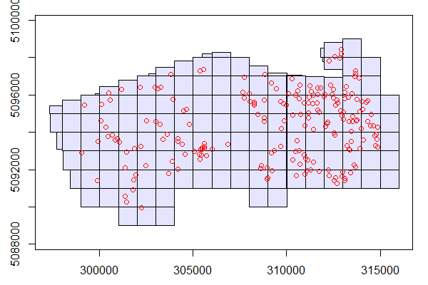
We have now prepared both our ALS and plot inventory data and can begin ABA processing.
Set opt_output_files option to write the results on disc. This is an important option to set. The clipped plots will be saved on hdd and not kept in memory. We also use the opt_filter function to ignore noise below 0 m so that they do not influence future processing.
# Write files to disc
opt_output_files(ctg) <- paste0(tempdir(), "/{PlotID}")

# Ignore points with elevations less than 0
opt_filter(ctg) <- "-drop_z_below 0"Note that the radius parameter is 14.1 because our plot radius is 14.1 m. This step may take a while but is fast if the point cloud is index with lax files .
# Clip catalog object using plots with a circular buffer of 14.1 m
plots_ALS_clipped <- clip_roi(ctg, plots, radius=14.1)
The plots_ALS_clipped object is now a LAScatalog object containing all clipped plots.
plots_ALS_clipped

#> class       : LAScatalog
#> extent      : 299037.3 , 314863.4 , 5089938 , 5098440 (xmin, xmax, ymin, ymax)
#> coord. ref. : +proj=utm +zone=18 +ellps=GRS80 +towgs84=0,0,0,0,0,0,0 +units=m +no_defs
#> area        : 160376.5 m²
#> points      : 1.67 million points
#> density     : 10.4 points/m²
#> num. files : 203 We first set some processing options using opt_chunk_buffer and opt_chunk_size. Setting these options to 0 mean that there will be no buffer around our plots when we calculate metrics and that processing will not be done in chunks (we do this for plots because they are small and do not require chunk processing functionality). We also use opt_output_files to have plot metrics stored in memory instead of on disc.
opt_chunk_buffer(plots_ALS_clipped) <- 0
opt_chunk_size(plots_ALS_clipped) <- 0
opt_output_files(plots_ALS_clipped) <- ""
To calculate metrics for each plot we use the catalog_apply() functionality. We specify that we want to process our plots_ALS_clipped catalog object using cloud_metrics() to calculate all metrics contained in the .stdmetrics_z function. The func argument also supports user defined functions. The output of catalog_apply() is a list of vectors (plots_metrics), which we convert into a data.table.
plots_metrics <- catalog_apply(plots_ALS_clipped, cloud_metrics, func = .stdmetrics_z)
plots_metrics <- data.table::rbindlist(plots_metrics)
We have now calculated a variety of ALS metrics for each plot. In order to complete our inventory and begin modelling we now must merge ALS metrics with field measured values (D).
D <- cbind(as.data.frame(plots), plots_metrics)Here we provide a simple example of how to create an OLS model (lm) for Lorey's Mean Height (HL). Using the summary and plot functions we found that the 85th percentile of height (zq85) for ALS metrics explain a large amount of variation in HL values. We are more than happy with this simple model.
m <- lm(HL ~zq85, data=D)
summary(m)

#> Call:
#> lm(formula = HL ~ zq85, data = D)
#>
#> Residuals:
#>    Min     1Q Median     3Q    Max
#> -4.640 -1.053 -0.031  1.030  4.258
#>
#> Coefficients:
#>             Estimate Std. Error t value Pr(>|t|)
#> (Intercept)  2.29496    0.31116   7.376  4.2e-12 ***
#> zq85         0.93389    0.01525  61.237  < 2e-16 ***
#> ---
#> Signif. codes:  0 ‘***’ 0.001 ‘**’ 0.01 ‘*’ 0.05 ‘.’ 0.1 ‘ ’ 1
#>
#> Residual standard error: 1.5 on 201 degrees of freedom
#> Multiple R-squared:  0.9491,	Adjusted R-squared:  0.9489
#> F-statistic:  3750 on 1 and 201 DF,  p-value: < 2.2e-16
Here we visualize the relationship between the observed (measured) and predicted (ALS-based) HL values.
plot(D$HL, predict(m))
abline(0,1)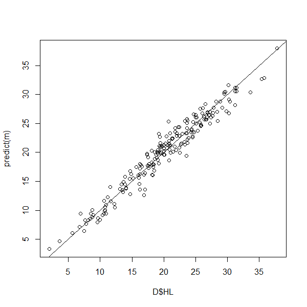
Now that we have created a model using plot data, we now need to apply that model across our entire study area.
To do so we first need to generate the same suite of ALS metrics (.stdmetrics_z) for our ALS data using the grid_metrics function on our original ctg LAScatalog object . We have chosen to write these metrics into memory. Note that the res parameter is set to 25 because we want the resolution of our metrics to match the area of our sample plots (14.1 m radius ≈ 625m2).
opt_output_files(ctg) <- ""
metrics_w2w <- grid_metrics(ctg, .stdmetrics_z, res = 25)
To visualize any of the metrics you can use the plot function.
plot(metrics_w2w$zq85)
plot(metrics_w2w$zmean)
plot(metrics_w2w$pzabovezmean)We can use two methods for applying our model (m) to all of our ALS data. We can do this manually using the model coefficients, or use the predict function. Both of these methods produce the same output (HL_pred) which is a wall-to-wall raster of predicted Lorey's mean height.
HL_pred <- coef(m)[1] + metrics_w2w$zq85 * coef(m)[2]
# or
HL_pred <- predict(metrics_w2w$zq85, m)
To visualize wall-to-wall predictions use
plot(HL_pred)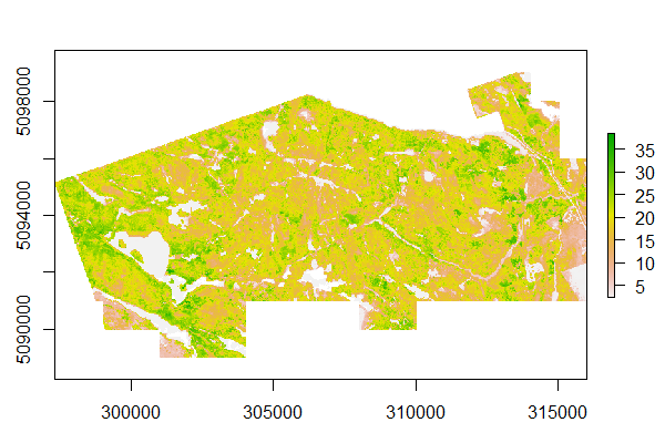
You're all done! Wow! Who knew ALS processing could be so easy, fun, and powerful using R!