Enrichment-Analysis

R code for getting from RNA-seq raw count to biological pathways (read on BioSatrs)

Introduction

Assume we performed an RNA-seq (or microarray gene expression) experiment and now want to know what pathway/biological process shows enrichment for our [differentially expressed] genes. There are terminologies someone may need to be familiar with before diving into the topic thoroughly:

Gene set

A gene set is an unordered collection of genes that are functionally related.

Pathway

A pathway can be interpreted as a gene set by ignoring functional relationships among genes.

Gene Ontology (GO)

GO describe gene function. A gene role/function could be attributed to the three main classes:

• Molecular Function (MF) : which defines molecular activities of gene products.

• Cellular Component (CC) : which describes where gene products are active/localized.

• Biological Process (BP) : which describes pathways and processes that the gene product is active in.

Kyoto Encyclopedia of Genes and Genomes (KEGG)

KEGG is a collection of manually curated pathway maps representing molecular interaction and reaction networks.

There are different methods widely used for functional enrichment analysis:

1- Over Representation Analysis (ORA):

This is the simplest version of enrichment analysis and at the same time the most widely used approach. The concept in this approach is based on a Fisher exact test p-value in a contingency table. For example, suppose we come up with 160 differentially expressed genes from a microarray expression experiment which was able to investigate 17,000 gene expression levels. We found that 30 genes from our findings are somehow a member of a pathway which has 50 gene members (call it pathway X). To find enrichment we can perform a Fisher exact test on the following contingency table:

	not.intrested.genes	intrested.genes
in pathwayX	20	30
not.in pathwayX	16820	130

There is a relatively large number of web-tools R package for ORA. Personally I am a fan of DAVID webtools for ORA.  

It is happening to me to have a list of genes and want to know what are common GO terms (usually BP) for these genes regardless of statistical significance. The package clusterProfiler provides a function groupGO that can be used to answer these kinds of questions. Here is how this function works:

#________________GO_Classification_____________________#
library(org.Hs.eg.db)
library(clusterProfiler)

# some genes from bladder cancer classification panel! 
geneList <- c("KRT14", "KRT5", "CDH3", "FOXA1", "GATA3", "PPARG", "RB1" , "CCND1", "CDKN2Ap16", "FGFR3", "TP63")

# convering gene symbol to gene ENTREZ ID
gene.df <- bitr(geneList, fromType = "SYMBOL",
                toType = c("ENSEMBL","ENTREZID" ),
                OrgDb = org.Hs.eg.db)
# GO classification,to read more about arguments used in this function please use ?groupGO to see help page
ggo <- groupGO(gene     = gene.df$ENTREZID,
               OrgDb    = org.Hs.eg.db,
               ont      = "BP",
               level    = 3,
               readable = TRUE)

ggo_df <- data.frame(ggo)

# This will return a table like this: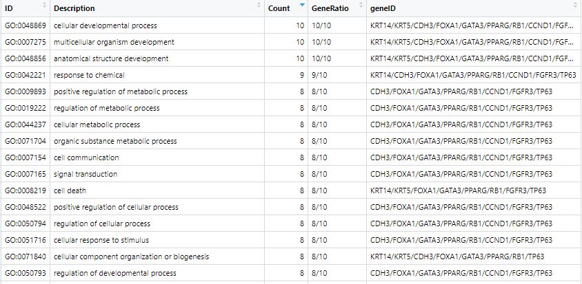

2- Gene Set Enrichment Analysis (GSEA):

It was developed by Broad Institute. This is the preferred method when genes are coming from an expression experiment like microarray and RNA-seq. However, the original methodology was designed to work on microarray but later modification made it suitable for RNA-seq also. In this approach, you need to rank your genes based on a statistic (like what DESeq2 provide), and then perform enrichment analysis against different pathways (= gene set). You have to download the gene set files into your local system. The point is that here the algorithm will use all genes in the ranked list for enrichment analysis. [in contrast to ORA where only genes passed a specific threshold (like DE ones) would be used for enrichment analysis]. You can find more details about the methodology on the original PNAS paper, here is a summary of why one should use this approach instead of ORA:

1- After correcting for multiple hypotheses testing, no individual gene may meet the threshold for statistical significance.

2- On the other hand, one may be left with a long list of statistically significant genes without any unifying biological theme.

3- Cellular processes often affect sets of genes acting in concert, using ORA may lead to miss important effects on pathways.

GSEA software maybe finds on its homepage. However, there are some Bioconductor packages that use a similar approach to do GSEA, I like to use this one : fgsea. Also, there is some R packages that can do ROA and GSEA for you like clusterProfiler.

In the analysis after getting a ranked gene from differential expression analysis, we need to have gene lists for GSEA. The Molecular Signatures Database (MSigDB) is a collection of annotated gene sets for use with GSEA software and possibly those works like GSEA. The MSigDB gene sets are divided into 9 major collections:

H: hallmark gene sets are coherently expressed signatures derived by aggregating many MSigDB gene sets to represent well-defined biological states or processes.

C1: positional gene sets for each human chromosome and cytogenetic band.

C2: curated gene sets from online pathway databases, publications in PubMed, and knowledge of domain experts.

C3: regulatory target gene sets based on gene target predictions for microRNA seed sequences and predicted transcription factor binding sites.

C4: computational gene sets defined by mining large collections of cancer-oriented microarray data.

C5: ontology gene sets consist of genes annotated by the same ontology term.

C6: oncogenic signature gene sets defined directly from microarray gene expression data from cancer gene perturbations.

C7: immunologic signature gene sets defined directly from microarray gene expression data from immunologic studies.

C8: cell type signature gene sets curated from cluster markers identified in single-cell sequencing studies of human tissue.

To download these gene sets in a folder go to the MSigDB website, register with your email, and download the data. Here first we should do a (1)differential expression analysis, then doing (2) GSEA and finally (3) Visualization.

#_______________Loading packages______________________________#
library(DESeq2)
library(org.Hs.eg.db)
library(tibble)
library(dplyr)
library(tidyr)
library(fgsea)
library(ggplot2)
library(reshape2)
library(ComplexHeatmap)
library(circlize)

 
#________________diffrential expression analysis______________#
# reading expression data matrix and getting rid of what we dont like

# my data is raw count data comming from RNA-seq on 476 bladder cancer sample
rna <- read.table("Uromol1_CountData.v1.csv", header = T, sep = ",")

dim(rna)
#  [1] 60488   477
head(rna, 5)

#  genes               U0001 U0002 U0006 U0007 U0010 U0011 U0012 U0013 U0015 U0018 U0023 U0024 U0026 U0027 U0028
#1 ENSG00000000003.13  1458   228  1800  3945   293  1737  6362  8869  1728  4822  5913   103  2138  4196  4949
#2 ENSG00000000005.5     0     0     9     0     0     0     0     5     2     2     2     0     2     4     2

# setting row name for expression matrix
rownamefordata <- substr(rna$genes,1,15)
rownames(rna) <- rownamefordata
rm(rownamefordata)
# removing column with gene name
rna <- rna[, -1]

# reading clinical data 
# read uromol clinical
uromol_clin <- read.table("uromol_clinic.csv", sep = ",", header = T)
names(uromol_clin)

#[1] "UniqueID"                           "CLASS"                              "BASE47"                            
#[4] "CIS"                                "X12.gene.signature"                 "Lund"                              
#[7] "Stage"                              "Grade"                              "EORTC.risk.score..NMIBC."          
#[10] "sex"                                "age"                                "TumorSize"                         
#[13] "GrowthPattern"                      "BCGTreatment"                       "CIS.in.disease.course"             
#[16] "Cystectomy"                         "Progression.to.T2."                 "Progression.free.survival..months."

#Setting row name for clinical data
ids <- uromol_clin$UniqueID
rownames(uromol_clin) <- ids
rm(ids)

# I want to compare samples with Ta stage against those in higher stage (non_Ta)
# making column for comparison

table(uromol_clin$Stage)

# CIS   T1 T2-4   Ta 
# 3     112   16  345 

# selecting only Ta samples
uromol_clin$isTa <- as.factor(ifelse(uromol_clin$Stage == "Ta", "Ta", "non_Ta"))
levels(uromol_clin$isTa)
# [1] "non-Ta" "Ta" 

# making sure dataset are compatible regrding to sample order
rna <- rna[, row.names(uromol_clin)]
all(rownames(uromol_clin) %in% colnames(rna))

#_______Making_Expression_Object__________#
#Making DESeqDataSet object which stores all experiment data
dds <- DESeqDataSetFromMatrix(countData = rna,
                              colData = uromol_clin,
                              design = ~ isTa)

# prefilteration: it is not necessary but recommended to filter out low expressed genes
keep <- rowSums(counts(dds)) >= 10
dds <- dds[keep,]
rm(keep)
# data tranfromation
vsd <- vst(dds, blind=FALSE)

#________________DE_analysis_____________#
dds <- DESeq(dds) #This would take some time
res <- results(dds, alpha=0.05)
summary(res)

#_________________GSEA___________________#
# Steps toward doing gene set emrichment analysis (GSEA):

# 1- obtaining a stats for ranking genes in your experiment,
# 2- creating a named vector out of the DESeq2 result
# 3- Obtaining a gene set from mysigbd
# 4- doing analysis


# already we performed DESeq2 analysis and have statitics for workig on it
res$row <- rownames(res)

# important notice: if you have not such stats in your result (say comming from edgeR),
# you may need to create a rank metric for your genes. To do this:
# metric = -log10(pvalue)/sign(log2FC)



# Map Ensembl gene IDs to symbol. First create a mapping table.
ens2symbol <- AnnotationDbi::select(org.Hs.eg.db,
                                    key=res$row, 
                                    columns="SYMBOL",
                                    keytype="ENSEMBL")
names(ens2symbol)[1] <- "row"

ens2symbol <- as_tibble(ens2symbol)
ens2symbol
# joining
res <- merge(data.frame(res), ens2symbol, by=c("row"))

# remove the NAs, averaging statitics for a multi-hit symbol
res2 <- res %>% 
  dplyr::select(SYMBOL, stat) %>% 
  na.omit() %>% 
  distinct() %>% 
  group_by(SYMBOL) %>% 
  summarize(stat=mean(stat))
res2

# creating  a named vector [ranked genes]
ranks <- res2$stat
names(ranks) <- res2$SYMBOL


# Load the pathway (gene set) into a named list
# downloaded mysigdb were located in my "~" directory:
pathways.hallmark <- gmtPathways("~/mysigdb/h.all.v7.2.symbols.gmt")

# show few lines from the pathways file
head(pathways.hallmark)

#Running fgsea algorithm:
fgseaRes <- fgseaMultilevel(pathways=pathways.hallmark, stats=ranks)

# Tidy the results:
fgseaResTidy <- fgseaRes %>%
  as_tibble() %>%
  arrange(desc(NES)) # order by normalized enrichment score (NES)

# To see what genes are in each of these pathways:
gene.in.pathway <- pathways.hallmark %>% 
  enframe("pathway", "SYMBOL") %>% 
  unnest(cols = c(SYMBOL)) %>% 
  inner_join(res, by="SYMBOL")

#______________________VISUALIZATION______________________________#

#__________bar plot _______________#
# Plot the normalized enrichment scores. 
#Color the bar indicating whether or not the pathway was significant:
fgseaResTidy$adjPvalue <- ifelse(fgseaResTidy$padj <= 0.05, "significant", "non-significant")
cols <- c("non-significant" = "grey", "significant" = "red")
ggplot(fgseaResTidy, aes(reorder(pathway, NES), NES, fill = adjPvalue)) +
  geom_col() +
  scale_fill_manual(values = cols) +
  theme(axis.text.x = element_text(angle = 90, vjust = 0.5, hjust=1)) +
  coord_flip() +
  labs(x="Pathway", y="Normalized Enrichment Score",
  title="Hallmark pathways Enrichment Score from GSEA")

#__________Enrichment  Plot_______#
# Enrichment plot for E2F target gene set
plotEnrichment(pathway = pathways.hallmark[["HALLMARK_E2F_TARGETS"]], ranks)

#
plotGseaTable(pathways.hallmark[fgseaRes$pathway[fgseaRes$padj < 0.05]], ranks, fgseaRes, 
                gseaParam=0.5)

#________ Heatmap Plot_____________#
# pathways with significant enrichment score
sig.path <- fgseaResTidy$pathway[fgseaResTidy$adjPvalue == "significant"]
sig.gen <- unique(na.omit(gene.in.pathway$SYMBOL[gene.in.pathway$pathway %in% sig.path]))

### create a new data-frame that has '1' for when a gene is part of a term, and '0' when not
h.dat <- dcast(gene.in.pathway[, c(1,2)], SYMBOL~pathway)
rownames(h.dat) <- h.dat$SYMBOL
h.dat <- h.dat[, -1]

h.dat <- h.dat[rownames(h.dat) %in% sig.gen, ]
h.dat <- h.dat[, colnames(h.dat) %in% sig.path]

# keep those genes with 3  or more occurnes
table(data.frame(rowSums(h.dat)))

# 1       2    3    4    5    6 
# 1604  282   65   11    1    1 
h.dat <- h.dat[data.frame(rowSums(h.dat)) >= 3, ]

#
topTable <- res[res$SYMBOL %in% rownames(h.dat), ]
rownames(topTable) <- topTable$SYMBOL

# match the order of rownames in toptable with that of h.dat
topTableAligned <- topTable[which(rownames(topTable) %in% rownames(h.dat)),]
topTableAligned <- topTableAligned[match(rownames(h.dat), rownames(topTableAligned)),]
all(rownames(topTableAligned) == rownames(h.dat))

# colour bar for -log10(adjusted p-value) for sig.genes
dfMinusLog10FDRGenes <- data.frame(-log10(
 topTableAligned[which(rownames(topTableAligned) %in% rownames(h.dat)), 'padj']))
dfMinusLog10FDRGenes[dfMinusLog10FDRGenes == 'Inf'] <- 0

# colour bar for fold changes for sigGenes
dfFoldChangeGenes <- data.frame(
 topTableAligned[which(rownames(topTableAligned) %in% rownames(h.dat)), 'log2FoldChange'])

# merge both
dfGeneAnno <- data.frame(dfMinusLog10FDRGenes, dfFoldChangeGenes)
colnames(dfGeneAnno) <- c('Gene score', 'Log2FC')

dfGeneAnno[,2] <- ifelse(dfGeneAnno$Log2FC > 0, 'Up-regulated',
                        ifelse(dfGeneAnno$Log2FC < 0, 'Down-regulated', 'Unchanged'))
colours <- list(
 'Log2FC' = c('Up-regulated' = 'royalblue', 'Down-regulated' = 'yellow'))
haGenes <- rowAnnotation(
 df = dfGeneAnno,
 col = colours,
 width = unit(1,'cm'),
 annotation_name_side = 'top')

# Now a separate colour bar for the GSEA enrichment padj. This will 
# also contain the enriched term names via annot_text()

# colour bar for enrichment score from fgsea results
dfEnrichment <- fgseaRes[, c("pathway", "NES")]
dfEnrichment <- dfEnrichment[dfEnrichment$pathway %in% colnames(h.dat)]
dd <- dfEnrichment$pathway
dfEnrichment <- dfEnrichment[, -1]
rownames(dfEnrichment) <- dd

colnames(dfEnrichment) <- 'Normalized\n Enrichment score'
haTerms <- HeatmapAnnotation(
 df = dfEnrichment,
 Term = anno_text(
   colnames(h.dat),
   rot = 45,
   just = 'right',
   gp = gpar(fontsize = 12)),
 annotation_height = unit.c(unit(1, 'cm'), unit(8, 'cm')),
 annotation_name_side = 'left')

# now generate the heatmap
hmapGSEA <- Heatmap(h.dat,
                   name = 'GSEA hallmark pathways enrichment',
                   split = dfGeneAnno[,2],
                   col = c('0' = 'white', '1' = 'forestgreen'),
                   rect_gp = gpar(col = 'grey85'),
                   cluster_rows = TRUE,
                   show_row_dend = TRUE,
                   row_title = 'Top Genes',
                   row_title_side = 'left',
                   row_title_gp = gpar(fontsize = 11, fontface = 'bold'),
                   row_title_rot = 90,
                   show_row_names = TRUE,
                   row_names_gp = gpar(fontsize = 11, fontface = 'bold'),
                   row_names_side = 'left',
                   row_dend_width = unit(35, 'mm'),
                   cluster_columns = TRUE,
                   show_column_dend = TRUE,
                   column_title = 'Enriched terms',
                   column_title_side = 'top',
                   column_title_gp = gpar(fontsize = 12, fontface = 'bold'),
                   column_title_rot = 0,
                   show_column_names = FALSE,
                   show_heatmap_legend = FALSE,
                   clustering_distance_columns = 'euclidean',
                   clustering_method_columns = 'ward.D2',
                   clustering_distance_rows = 'euclidean',
                   clustering_method_rows = 'ward.D2',
                   bottom_annotation = haTerms)

tiff("GSEA_enrichment_2.tiff", units="in", width=13, height=22, res=400)
draw(hmapGSEA + haGenes,
    heatmap_legend_side = 'right',
    annotation_legend_side = 'right')
dev.off()

Session Info

Refrences

1- clusterProfiler: universal enrichment tool for functional and comparative study

2- Fast Gene Set Enrichment Analysis

3- Gene set enrichment analysis: A knowledge-based approach for interpreting genome-wide expression profiles

4- DAVID Bioinformatics Resources 6.8

5- DESeq results to pathways in 60 Seconds with the fgsea package

6- Rank-rank hypergeometric overlap: identification of statistically significant overlap between gene-expression signatures

7- Clustering of DAVID gene enrichment results from gene expression studies by Kevin Blighe