Virtual Gyro

In Rotations and Orientations Part 1 and Part 2, we explored some of the mathematical ways to represent the orientation of an object. Now we’re going to apply that knowledge to build a virtual gyroscope using data from a 3-axis accelerometer and 3-axis magnetometer. Reasons you might want to do this include “cost” and “cost”. Cost #1 is financial. Gyros tend to be more expensive than the other two sensors. Eliminating them from the BOM is attractive for that reason. Cost #2 is power. The power consumed by a typical accel/mag pair is significantly less than that consumed by a MEMS gyro. The downside of a virtual gyro is that it is sensitive to linear acceleration and uncorrected magnetic interference. If either of those is present, you probably still want a physical gyro.

So how do we go from orientation to angular rates? It’s conceptually easy if you step back and consider the problem from a high level. Angular rate can be defined as change in orientation per unit time. We already know lots of ways to model orientation. Figure out how to take the derivative of the orientation and we’re there!

In the prior postings, we’ve discussed a number of ways to represent orientation. For this discussion, we will use the basic rotation matrix. Jack B. Kuipers has a nice derivation of the derivative of direction cosine matrices in his “Quaternions and Rotation Sequences” text - one of my most used textbooks. It makes a good starting point. Paraphrasing his math:

Let:

Expresson	Equation Number
vf = some vector v measured in a fixed reference frame	Eqn 1
vb = same vector measured in a moving body frame	Eqn 2
RMt = rotation matrix which takes vf into vb	Eqn 3
ω = angular rate through the rotation	Eqn 4

Then at any time t:

Expresson	Equation Number
vb= RMt vf	Eqn 5

Differentiate both sides (use the chain rule on the RHS):

Expresson	Equation Number
dvb/dt = (dRMt/dt) vf + RMt(dvf/dt)	Eqn 6

Our restrictions on no linear acceleration or magnetic interference imply that:

Expresson	Equation Number
dvf/dt = 0	Eqn 7

Then:

Expresson	Equation Number
dvb/dt = (dRMt/dt) vf	Eqn 8

We know that:

Expresson	Equation Number
vf = RMt-1 vb	Eqn 9

Plugging this into (8) yields

Expresson	Equation Number
dvb/dt = (dRMt/dt) RMt-1 vb	Eqn 10

In a previous posting (Accelerometer placement - where and why , we learned about the transport theorem, which describes the rate of change of a vector in a moving frame:

Expresson	Equation Number
dvf/dt = dvb/dt - ω X vb	Eqn 11

Those who take the time to check will note that we have inverted the polarity of the ω in Equation 11 from that shown in the prior posting. In that case ω was the angular velocity of the body frame in the fixed reference frame. Here we want it from the opposite perspective (which would match gyro outputs).

And again,

Expresson	Equation Number
dvf/dt = 0	Eqn 12
so

Expresson	Equation Number
dvb/dt = ω X vb	Eqn 13

Equating equations 10 and 13:

Expresson	Equation Number
ω X vb = (dRMt/dt) RMt-1 vb	Eqn 14
ω X = (dRMt/dt) RMt-1	Eqn 15

where:

Expresson	Equation Number
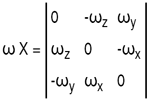	Eqn 16

Going back to the fundamentals in our first calculus course and using a one-sided approximation to the derivative:

Expresson	Equation Number
dRMt/dt = (1/Δt)(RMt+1 – RMt)	Eqn 17

where Δt = the time between orientation samples

Expresson	Equation Number
ωb X = (1/Δt)(RMt+1 – RMt) RMt-1	Eqn 18

Recall that for rotation matrices, the transpose is the same as the inverse:

Expresson	Equation Number
RMtT = RMt-1	Eqn 19
ωb X = (1/Δt)(RMt+1 - RMt) RMtT	Eqn 20

Equation 20 is a truly elegant equation. It shows that you can calculate angular rates based upon knowledge of only the last two orientations. That makes perfect intuitive sense, and I’m ashamed when I think how long it took me to arrive at it the first time.

An alternate form that is even more attractive can be had by carrying out the multiplications on the RHS:

Expresson	Equation Number
ωb X = (1/Δt)(RMt+1 RMtT - RMt RMtT)	Eqn 21
ωb X = (1/Δt)(RMt+1 RMtT - I3x3)	Eqn 22

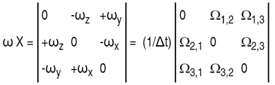
For the sake of being explicit, let’s expand the terms. A rotation matrix has dimensions 3x3. So both left and right hand sides of Eqn. 22 have dimensions 3x3.

Expresson	Equation Number
(1/Δt)(RMt+1 RMtT – I3x3) = (1/Δt) Ω	Eqn 23
	Eqn 24

The zero value diagonal elements in W result from small angle approximations since the diagonal terms on RMt+1 RMtT will be close to one, which will be canceled by the subtraction of the identity matrix. Then:

Expresson	Equation Number
	Eqn 25

and we have:

Expresson	Equation Number
ωx= (1/2Δt) (Ω3,2 - Ω2,3)	Eqn 26
ωy= (1/2Δt) (Ω1,3 - Ω3,1)	Eqn 27
ωz= (1/2Δt) (Ω2,1 - Ω1,2)	Eqn 28

Once we have orientations, we’re in a position to compute corresponding angular rates with

• One 3x3 matrix multiply operation
• 3 scalar subtractions
• 3 scalar multiplications at time each point. Sweet!

Some time ago, I ran a Matlab simulation to look at outputs of a gyro versus outputs from a "virtual gyro" based upon accelerometer/magnetometer readings. After adjusting for gyro offset and scale factors, I got pretty good correlation, as can be seen in the figure below.

You will notice that we started with an assumption that we already know how to calculate orientation given accelerometer/magnetometer readings. There are many ways to do this. I can think of three off the top of my head:

• Compute roll, pitch and yaw as described in Freescale AN4248. Use those values to compute rotation matrices as described in Orientation Representations: Part 1. This approach uses Euler angles, which I like to stay away from, but you could give it a go.
• Use the Android getRotationMatrix [4] to compute rotation matrices directly. This method uses a sequence of cross-products to arrive at the current orientation.
• Use a solution to Wahba’s problem to compute the optimal rotation for each time point.

Whichever technique you use to compute orientations, you need to pay attention to a few details: Remember that non-zero linear acceleration and/or uncorrected magnetic interference violate the physical assumptions behind the theory.

The expressions shown generally rely on a small angle assumption. That is, the change in orientation from one time step to the next is relatively small. You can encourage this by using a short sampling interval. It is possible to discard that assumption and deal with large angles directly, but the math isn't as intuitive.

Noise in the accelerometer and magnetometer outputs will result in very visible noise in the virtual gyro output. You will want to low pass filter your outputs prior to using them.

Respectfully submitted for your enjoyment,

Michael Stanley

References

• Freescale Application Note Number AN4248: Implementing a Tilt-Compensated eCompass using Accelerometer and Magnetometer Sensors
• Orientation Representations: Part 1 blog posting on the Embedded Beat
• Orientation Representations: Part 2 blog posting on the Embedded Beat
• getRotationMatrix() function defined at http://developer.android.com/reference/android/hardware/SensorManager.htmlWikipedia entry for "Wahba’s problem"
• U.S. Patent Application 13/748381, SYSTEMS AND METHOD FOR GYROSCOPE CALIBRATION, Michael Stanley, Freescale Semiconductor

Virtual Gyro by Freescale Semiconductor is licensed under a Creative Commons Attribution 4.0 International License.