Hillshade
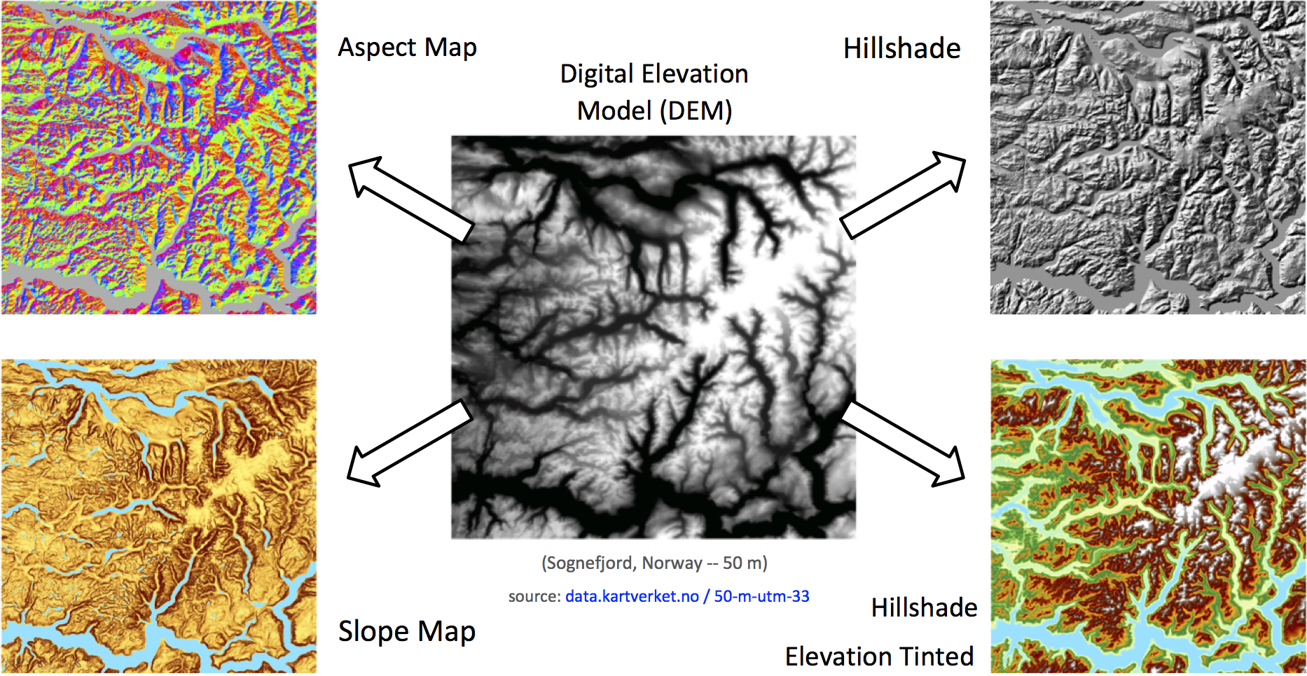
The following Python script computes the hillshade of a digital elevation model (DEM) following Horn’s formulation [1]. This algorithms draws a self-shadowing effect on top of a DEM according to some specific azimuth and altitude angles of the sun. Hillshade creates a sense of topographic relief, as if the DEM was a three-dimensional model with real shadows generated by the absence of sunlight.
A straightforward Hillshade script is listed below:
    from map import * ## Parallel Map Algebra
    PI = 3.141593

    def hori(dem, dist):
        h = [ [1, 0, -1],
              [2, 0, -2],
              [1, 0, -1] ]
        return convolve(dem,h) / 8 / dist

    def vert(dem, dist):
        v = [ [ 1, 2, 1],
              [ 0, 0, 0],
              [-1,-2,-1] ]
        return convolve(dem,v) / 8 / dist

    def slope(dem, dist=1):
        x = hori(dem,dist)
        y = vert(dem,dist)
        z = atan(sqrt(x*x + y*y))
        return z

    def aspect(dem, dist=1):
        x = hori(dem,dist)
        y = vert(dem,dist)
        z1 = (x!=0) * atan2(y,-x)
        z1 = z1 + (z1<0) * (PI*2)
        z0 = (x==0) * ((y>0)*(PI/2)
           + (y<0)*(PI*2-PI/2))
        return z1 + z0

    def hillshade(dem, zenith, azimuth):
        zr = (90 - float(zenith)) / 180*PI
        ar = 360 - float(azimuth) + 90
        ar = ar - 360 if (ar > 360) else ar
        ar = ar / 180 * PI
        hs = cos(zr) * cos(slope(dem)) +
             sin(zr) * sin(slope(dem)) *
             cos(ar - aspect(dem))
        return hs

    dem = read('in_file_path')
    out = hillshade(dem,45,315)
    write(out,'out_file_path')
The actual source file for the hillshade script can be found here.
When the Python script is executed the raster operations are not carried out immediately, but are instead used to extract a dependency graph. The graph is analyzed and the operations are fused according to their Map Algebra classes (Local,Focal,Zonal...) and their relation (e.g. producer-consumer).
Hillshade presents two Focal operations, the horizontal and vertical convolutions, while the rest are all Local operations. The Local pattern often fuses seamlessly and as a result the Hillshade script can be fused into a single group of nodes. This implies that all operations can be executed within one OpenCl kernel, which saves memory movements from/ to global memory. If the operations were not fused but executed in an interpreted fashion instead, the framework would need to execute many OpenCL kernels and would unnecessarily move the temporal resuls up and down the memory heirarchy.
The dependency graph is presented below. All the nodes fuse into the red group:
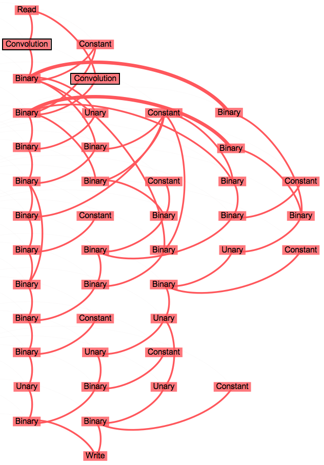
Groups inherit the Map Algebra classes from their nodes. The group above is of type Focal+Local and will execute following the most restrective algorithmic pattern, in this case the stencil pattern.
The framework includes algorithm skeletons to generate the parallel code. Obtaining the OpenCL kernel is therefore as simple as feeding the stencil skeleton with the group and storing the returned string, which will be compiled by the OpenCL drivers later on.
The generated OpenCL kernel code looks like this:
kernel void krn7515591183092765465
(
    TYPE_VAR_LIST(float,IN_43),
    int IN_45v,
    int IN_53v,
    float IN_57v,
    float IN_60v,
    int IN_62v,
    float IN_68v,
    float IN_73v,
    float IN_76v,
    float IN_81v,
    global float *OUT_85,
    const int BS0,
    const int BS1,
    const int BC0,
    const int BC1,
    const int GS0,
    const int GS1
)
{
    float F32_43, F32_57, F32_60, F32_68, F32_73, F32_76, F32_81, F32_44, F32_46,
          F32_47, F32_48, F32_49, F32_50, F32_51, F32_52, F32_54, F32_55, F32_56,
          F32_58, F32_59, F32_61, F32_64, F32_65, F32_66, F32_69, F32_70, F32_74,
          F32_77, F32_78, F32_79, F32_80, F32_82, F32_83, F32_84, F32_85;
    uchar U8_63, U8_67, U8_71, U8_72, U8_75;
    int S32_45, S32_53, S32_62;
    local float F32S_43[324];

    int gc0 = get_local_id(0);
    int gc1 = get_local_id(1);
    int bc0 = get_global_id(0);
    int bc1 = get_global_id(1);
    int H0 = 1;
    int H1 = 1;

    int S32L_44[3][3] = {{-1,0,1},{-2,0,2},{-1,0,1}};
    int S32L_47[3][3] = {{-1,-2,-1},{0,0,0},{1,2,1}};

    // Previous to FOCAL core

    if (bc0 < BS0 && bc1 < BS1) {
        for (int i=0; i<((GS1+2*H1)*(GS0+2*H0)-1)/(GS0*GS1)+1; i++)
        {
            int proj = (gc1)*GS0+gc0 + i*(GS0*GS1);
            if (proj >= (GS1+2*H1)*(GS0+2*H0)) continue;
            int gc0 = proj % ((GS0+2*H0)) / 1;
            int gc1 = proj % ((GS1+2*H1)*(GS0+2*H0)) / (GS0+2*H0);
            int bc0 = get_group_id(0)*GS0 + gc0 - H0;
            int bc1 = get_group_id(1)*GS1 + gc1 - H1;

            F32_43 = LOAD_F_F32(IN_43);
            F32S_43[(gc1)*(GS0+H0*2)+gc0] = F32_43;
        }
    }
    barrier(CLK_LOCAL_MEM_FENCE);

    // FOCAL core

    if (bc0 < BS0 && bc1 < BS1)
    {
        F32_44 = 0;
        for (int i1=-1; i1<=1; i1++) {
            for (int i0=-1; i0<=1; i0++) {
                F32_44 += LOAD_X_F32S(F32S_43) * LOAD_X_S32L(S32L_44);
            }
        }
        F32_47 = 0;
        for (int i1=-1; i1<=1; i1++) {
            for (int i0=-1; i0<=1; i0++) {
                F32_47 += LOAD_X_F32S(F32S_43) * LOAD_X_S32L(S32L_47);
            }
        }
    }

    // Posterior to FOCAL core

    if (bc0 < BS0 && bc1 < BS1) {
        F32_43 = LOAD_L_F32(IN_43);
        S32_45 = IN_45v;
        S32_53 = IN_53v;
        F32_57 = IN_57v;
        F32_60 = IN_60v;
        S32_62 = IN_62v;
        F32_68 = IN_68v;
        F32_73 = IN_73v;
        F32_76 = IN_76v;
        F32_81 = IN_81v;
        F32_46 = F32_44 / S32_45;
        F32_48 = F32_47 / S32_45;
        F32_49 = F32_46 * F32_46;
        F32_50 = F32_48 * F32_48;
        F32_51 = F32_49 + F32_50;
        F32_52 = sqrt(F32_51);
        F32_54 = S32_53 * F32_52;
        F32_55 = atan(F32_54);
        F32_56 = cos(F32_55);
        F32_58 = F32_57 * F32_56;
        F32_59 = sin(F32_55);
        F32_61 = F32_60 * F32_59;
        U8_63 = F32_46 != S32_62;
        F32_64 = -F32_46;
        F32_65 = atan2(F32_48,F32_64);
        F32_66 = U8_63 * F32_65;
        U8_67 = F32_66 < S32_62;
        F32_69 = U8_67 * F32_68;
        F32_70 = F32_66 + F32_69;
        U8_71 = F32_46 == S32_62;
        U8_72 = F32_48 > S32_62;
        F32_74 = U8_72 * F32_73;
        U8_75 = F32_48 < S32_62;
        F32_77 = U8_75 * F32_76;
        F32_78 = F32_74 + F32_77;
        F32_79 = U8_71 * F32_78;
        F32_80 = F32_70 + F32_79;
        F32_82 = F32_81 - F32_80;
        F32_83 = cos(F32_82);
        F32_84 = F32_61 * F32_83;
        F32_85 = F32_58 + F32_84;
        OUT_85[(bc1)*BS0+bc0] = F32_85;
    }
}
Large groups of nodes lead to large codes that give the OpenCL compiler more opportunities for low level optimizations such as register allocation, instruction scheduling/ selection or arithmetic simplification. Note how the convolution filters are defined statically in the kernel. Since this information is known by the compiler, it can unroll the convolution loops and optimize the operations aggressively.
Here is a dump of the assembly code generated by the Intel OpenCL compiler for a Skylake i7-6700 CPU. See the numerous fused-multiply-add operations, the vector-square-root and the calls to the Short Vector Math Library (SVML) to execute trigonometrics with the AVX2 ISA extension. Note also how the convolutions where fully unrolled and there is no sign of loop in the first part of the asm code. There is even a fused-sin-cos vector instruction. It is impressive that such high-quality low-level SIMD code was automatically generate from a Python script.
    . . .                                   - - - - ->
    vfmadd213ps %ymm0, %ymm1, %ymm9         |       vmulps  2464(%rbx), %ymm0, %ymm9
    vaddps  %ymm2, %ymm9, %ymm9                     vxorps  .LCPI1_15(%rip), %ymm15, %ymm1
    vbroadcastss    .LCPI1_13(%rip), %ymm10 |       vmovaps %ymm8, %ymm0
    vmovaps %ymm10, %ymm11                      --> callq   __ocl_svml_l9_atan2f8
    vfmadd213ps %ymm9, %ymm3, %ymm11        |       vcmpneqps   %ymm12, %ymm15, %ymm1
    vaddps  %ymm4, %ymm11, %ymm9                    vbroadcastss    .LCPI1_16(%rip), %ymm2
    vbroadcastss    .LCPI1_14(%rip), %ymm11 |       vandps  %ymm2, %ymm1, %ymm1
    vmovaps %ymm11, %ymm15                          vmulps  %ymm0, %ymm1, %ymm0
    vfmadd213ps %ymm9, %ymm5, %ymm15        |       vcmpltps    %ymm12, %ymm0, %ymm1
    vsubps  %ymm6, %ymm15, %ymm9                    vandps  %ymm2, %ymm1, %ymm1
    vxorps  %ymm15, %ymm15, %ymm15          |       vmovaps 2496(%rbx), %ymm3
    vfmadd213ps %ymm9, %ymm7, %ymm15                vfmadd213ps %ymm0, %ymm3, %ymm1
    vaddps  %ymm8, %ymm15, %ymm9            |       vcmpltps    %ymm8, %ymm12, %ymm0
    vfmadd213ps %ymm0, %ymm1, %ymm10                vandps  %ymm2, %ymm0, %ymm0
    vsubps  %ymm2, %ymm10, %ymm0            |       vcmpltps    %ymm12, %ymm8, %ymm3
    vfmadd213ps %ymm0, %ymm13, %ymm3                vandps  %ymm2, %ymm3, %ymm3
    vaddps  %ymm4, %ymm3, %ymm0             |       vmulps  2560(%rbx), %ymm3, %ymm3
    vfmadd213ps %ymm0, %ymm13, %ymm5                vmovaps 2528(%rbx), %ymm4
    vaddps  %ymm6, %ymm5, %ymm0             |       vfmadd213ps %ymm3, %ymm4, %ymm0
    vfmadd213ps %ymm0, %ymm7, %ymm11                vcmpeqps    %ymm12, %ymm15, %ymm3
    vmovaps 2400(%rbx), %ymm1               |       vandps  %ymm2, %ymm3, %ymm2
    vdivps  %ymm1, %ymm9, %ymm15                    vfmadd213ps %ymm1, %ymm0, %ymm2
    vaddps  %ymm8, %ymm11, %ymm0            |       vmovaps 2624(%rbx), %ymm0
    vdivps  %ymm1, %ymm0, %ymm8                     vsubps  %ymm2, %ymm0, %ymm0
    vmulps  %ymm8, %ymm8, %ymm0             |   --> callq   __ocl_svml_l9_cosf8
    vmovaps %ymm15, %ymm1                           movq    %r15, %r11
    vfmadd213ps %ymm0, %ymm1, %ymm1         |       vmulps  %ymm0, %ymm9, %ymm0
--> vsqrtps %ymm1, %ymm0                            movl    -128(%r11), %eax
    vmulps  2368(%rbx), %ymm0, %ymm0        |       imull   436(%rbx), %eax
--> callq   __ocl_svml_l9_atanf8                    vmovaps 2432(%rbx), %ymm1
    movq    %r15, %rdi                      |       vfmadd213ps %ymm0, %ymm1, %ymm10
--> callq   __ocl_svml_l9_sincosf8                  addl    -160(%r11), %eax
    vmovaps %ymm0, -32(%r15)                |       cltq
    vmovaps (%r15), %ymm10                          movq    440(%rbx), %rcx
    vpcmpeqd    %ymm2, %ymm2, %ymm2         |       vmovups %ymm10, (%rcx,%rax,4)
    vptest  %ymm2, %ymm14                           jmp .LBB1_80
    jae .LBB1_63                            |       . . .
- - - - - - - - - - - - - - - - - - - ->Now that we have the machine code, it can be finally executed with the input DEM to generate the output Hillshade. The image at the top of this page shows an example of input DEM, intermediate Aspect and Slope, final Hillshade and elevation colormap tinted by the hillshade. These rasters were visualized with ArcMap, since this project does not implement visualization routines.
[1] Horn BKP (1981) Hill shading and the reflectance map. Proc IEEE 69:14–47