Map Algebra is a mathematical formalism for the processing and analysis of raster geographical data (see "Geographic Information Systems and Cartographic Modelling," Tomlin 1990). Map Algebra becomes a powerful spatial modeling framework when embedded into a scripting language with branching, looping and functions.
Operations in Map Algebra only take and return rasters. They belong to one of several classes:
- Local: access single raster cells (element-wise/ map pattern)
- Focal: access bounded neighborhoods (stencil/ convolution pattern)
- Zonal: access any cell with associative order (reduction pattern)
- Global: access any cell following some particular topological order
- e.g. viewshed analysis, least cost analysis, hydrological modeling...
For my PhD I design a Parallel Map Algebra framework that runs efficiently on OpenCL devices. Users write sequential single-source Python scripts and the framework generates and executes kernel code automatically. Compiler techniques are at the core of system, from dependency analysis to loop fusion. They key challenge is maximizing data locality, since memory movements pose the major bottleneck to performance.
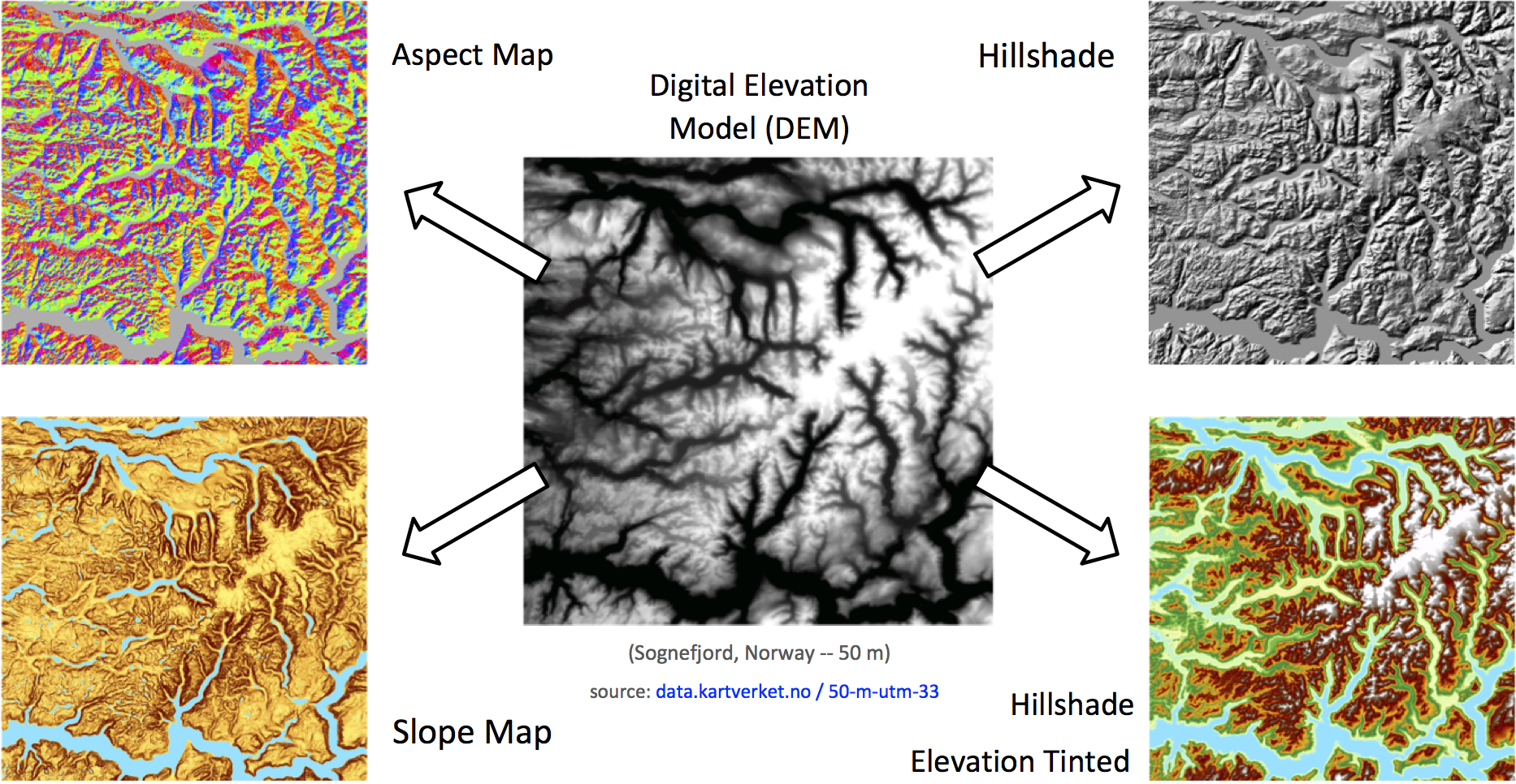
The following script depicts a hillshade algorithm. It computes and matches the derivatives of a DEM to the azimuth and altitude of the sun to achieve an effect of topographic relief.
    from map import * ## Parallel Map Algebra       # This is it, a Python import. Now the python script
    PI = 3.141593                                   # will execute the Map Algebra operations in parallel

    def hori(dem, dist):                            # Functions are just fine, the will be 'inlined' so that
        h = [ [1, 0, -1],                           # they don't get in the way of the auto-parallelization
              [2, 0, -2],
              [1, 0, -1] ]                          # Parallel convolutions (Focal Op) are easily applied to
        return convolve(dem,h) / 8 / dist           # the raster using a filter of NxM weights and 'convolve'

    def vert(dem, dist):                            # Raster copies like in 'd = dem' are optimized away
        d = dem
        v = 1*d(-1,-1) +2*d(0,-1) +1*d(1,-1)        # An alternative way of applying Focal Ops is through the
           +0*d(-1,0)  +0*d(0,0)  +0*d(1,0)         # __call__ operator and the relative neighbor coordinates
           -1*d(-1,1)  -2*d(0,1)  -1*d(1,1)         # This code is virtually similar to the convolution above,
        return v / 8 / dist                         # but it uses different weights (i.e. vertical derivative)

    def slope(dem, dist=1):
        x = hori(dem,dist)                          # Since functions are 'inlined', the framework can apply
        y = vert(dem,dist)                          # interprocedural optimizations between 'hori' and 'vert'
        z = atan(sqrt(x*x + y*y))
        return z                                    # 'returns' are optimized away; there is no copy of data

    def aspect(dem, dist=1):                        # We use Global Value Numbering (Click 95) and therefore
        x = hori(dem,dist)                          # interprocedural optimizations also happen in nested scopes
        y = vert(dem,dist)                          # e.g. when both 'slope' and 'aspect' call 'hori' and 'vert'
        z1 = (x!=0) * atan2(y,-x)
        z1 = z1 + (z1<0) * (PI*2)                   # Currently we employ a pure data flow model with no
        z0 = (x==0) * ((y>0)*(PI/2)                 # control flow graph, thus 'branching' is not possible.
           + (y<0)*(PI*2-PI/2))                     # The alternative is to use the con(bool,if,else) function
        return z1 + z0                              # or the boolean technique employed in the code to the left

    def hillshade(dem, zenith, azimuth):            # The framework applies ordinary compilers techniques:
        zr = (90 - float(zenith)) / 180*PI          # arithmetic simplification, constant folding/ propagation,
        ar = 360 - float(azimuth) + 90              # copy propagation, common subexpression elimination and
        ar = ar - 360 if (ar > 360) else ar         # dead code elimination. e.g. all this constants are folded.
        ar = ar / 180 * PI
        hs = cos(zr) * cos(slope(dem)) +            # Note how simply is the script, yet it generates parallel
             sin(zr) * sin(slope(dem)) *            # OpenCL kernel code that executes in powerful GPU devices.
             cos(ar - aspect(dem))
        return hs                                   # Oh, and memory is not a limitation, rasters larger than
                                                    # GPU memory can be processed seamlessly. For example,
    dem = read('in_file_path')                      # read(...) can open 1 TB nation-wide rasters w/o problem
    out = hillshade(dem,45,315)
    write(out,'out_file_path')                      # And finally we write the output results, the hillshade!
When the Python script is executes the operations are not carried out right away. Instead the framework composes a dependency graph, applies optimizations like fusion and generates OpenCL code. (See these steps here). Then the rasters are decomposed into blocks and the parallel code is executed as a batch of tasks.
The workflow of the framework is summarized in the following points:
- A user writes a sequential python script composed of map algebra operations.
- A symbolic representation in the form of dependency graph is derived from the script.
- Simplification routines optimize the graph. Then fusion groups consecutive operations.
- The graph is translated to OpenCL kernel code using algorithmic skeletons.
- The kernel code is compiled to device code, which is used to compose tasks.
- Spatial decomposition is applied to the raster data, resulting in blocks of cells.
- The pair {task, block} forms a job, the unit of execution and scheduling.
- Jobs are put into a work queue and a scheduler reorders them to maximize locality.
- An in-memory cache keeps the blocks at the higher levels of the memory hierarchy.
- Executing active jobs produces new blocks, which enables following jobs for execution.
- Concurrent worker threads handle the scheduler, cache, I/O and jobs until all work is done.
If you wish to know more about the approach, go have a look to the scripts and explanations in the wiki:
- Compiler approach to Parallel Map Algebra
- Hillshade extended, Statistics i.e. mean/max/std, Viewshed analysis, Conway's Game of Life
- Cellular Automata for Urban Growth
- Cellular Automata for Water Flow
- ...
Note: this is a research project and the code is only a prototype for testing our research hypothesis. If you got questions, contact me through email!
Jesús Carabaño Bravo jcaraban@abo.fi | PhD Student at Åbo Akademi, Finland