Digital Twin of Anthropomorphic Robotic Arm using AR

As the global manufacturing industry enters its fourth revolution, innovations such as robotics, automation, and artificial intelligence (AI) are set to take over. The number of active industrial robots worldwide is increasing by approximately 14% year on year, and automation creates new types of robots with improved utility and function. Factories of the future will likely feature robots and humans working side-by-side to meet consumer demand—a new world for which business owners should be prepared.

Based on current projections, AI is expected to have the ability to increase labor productivity by up to 40% by 2035, and robots are generally designed to take on repetitive tasks and allow workers to focus on more intensive duties. A major benefit of robots in automating large manufacturing operations is that some tasks could effectively be completed 24/7, thereby boosting production output without any additional labor costs.

RT Knits Ltd bought a 6dof robot to retrieve garments from printing machines in the Printing Department. It is the first robot of the brand Borunte which the company invested in. Hence, I wanted to take this opportunity to explore the mathematical and physical models of a 6-axis industrial robot and build a Digital Twin of the machine for simulation of future processes.

Through this project, I want to provide a basic understanding of how robots work and develop models to control them. We will find many different kinds of robots with different axes and different mechanical configurations in the industry. However, the 6-axes one is the most commonly used, and also, it is one of the most complicated ones. Hence, if we understand how this one works, we should be able to solve models for all the others.

Abstract

Simulation is an extremely important part of the development of a robot, and in general of any kind of industrial machine or process. Creating a simulated version of our machine, a so-called digital twin, will give you many advantages:

Model Validation: We can validate the correctness of our model. For example, after we write the inverse kinematics of our robot we can check that the results are correct in simulation, before we go on the real machine. This makes testing much safer and cheaper.
Design Planning: We can also plan and optimize our entire production line design. In simulation we can make sure our robots are in the best position to avoid singularities and have time-optimal trajectories for the tasks to be completed.
Process Monitoring: We can remotely connect the simulation to the real machine, and control it or simply view it from our office.

The main goal of this project is to understand the mathematical concepts behind a standard 6-axes industrial manipulator and build a Digital Twin in Unity which will allow us to simulate any other tasks.

A special thanks to Prof. Fabrizio for the guidance on this project. Most of the concepts explained below are based on his materials.

Plan of Action

Research on Industrial Robots
Coordinate Frames and Vectors
Forward Kinematics
Inverse Kinematics
Path Planning
Workspace Monitoring
Trajectory Generation
Mechanics
Implementation

1. Industrial Robots

Most industrial robots are mechanical arms controlled by electric servo motors and programmed to perform a specific task. This task is mainly repetitive, tedious and boring such that robots are more fitted to perform these tasks than humans. It is important to note here that these robots only perform actions that it was programmed for and does not utilizes any form of intelligence. It has no visual inputs and no AI that can allow it to take decisions on the go. However, a lot of research is being done that uses Reinforcement Learning so that the robot teaches itself to perform task such as grabbing objects of different sizes and shapes.

Fig. Industrial robots in automobile industry.

Constituting of mechanical arms, the industrial robots can lift objects ranging from 1Kg to 400 Kg. The mechanical arm robots can be found in all sorts of factories but they are mainly suited in metal working and automobile industry for cutting, painting, welding and assembling tasks. At RT Knits, we will use the robot for packaging, palletizing and handling of goods.

Industrial robots differ in various configurations however, they can further be segmented into two main parts: Serial Kinematic and Paralell Kinematic.

1.1 Serial Kinematic

Serial kinematics consists of an open chain of links similar to the human arm. The should, arm, wrists and fingers all form a chain of links and joints. This configuration is normally used for higher payloads and have a much more flexibility to reach a desired target location with more than one possible orientations. The flexibility is measured w.r.t the number of degrees of freedom(dof). Our robotic arm has 6 dof: 3 in position and 3 in orientation. Serial kinematics also allows for larger workspaces such that the robot can reach object far from its base. However, their two main disadvantage sare that they are slower and less accurate than the paralell kinematic system. This happends because each link adds some weight and errors to the chain hence, the total error is cummulative of the number of joints. It is possible to build a robot with more joints however, we also increases the complexity to control the entity.

Fig. Da Vinci's drawing of human arm(left) and Serial kinematic drawing of robotic arm(right).

To sum up about Serial Kinematics:

Higher payloads(5 Kg - 300 Kg)
Higher number of dof
Larger workspace
Slower movements
Lower accuracy

1.2 Paralell Kinematic

In a paralell manipulator, the actuated joints are not all attached to the ends of the other actuated joints. Instead the actuated joints are placed in paralell such that each joint is connected both to the end-effector and to the ground in the manipulator. This configuration is mainly used in setting where the payload to be lifted is lower(<10Kg) and the required dof is only 3 or 4. However, there exists robots which can lift higher payloads and have 6 dof such as the Gough-Stewart platform but these are not common in industrial setting. In contrast to serial kinematics, paralell manipulators have a limited workplace but can move much faster and have a higher accuracy because errors do not add up between joints.

Fig. Figure shows 6 actuated joints connected in paralell.

To sum up about paralell kinematic:

Lower payload(<10 Kg)
Fewer dof
Smaller workplace
Faster movements
Higher accuracy

The video below shows the distinction between serial and paralell manipulators.

KINEMATICS._.Serial.robot.vs.Parallel.robot.This.is.not.CGI.mp4

Fig 1. ([Video by Oleksandr Stepanenko](https://www.youtube.com/watch?v=3fbmguBgVPA))

1.3 6-axis Anthropomorphic Robotic Arm

Our 6-axis robot is a serial kinematic structure with 6 links connected together by 6 joints. The robot starts with a base fixed to the ground. It has a motor underneath to allow rotation in the horizontal plane. It has a first axis connected to the base to allow the rotation motion - it is called J1 which stands for Joint 1. Then we have a second and a third axis called J2 and J3. Note here that J1, J2 and J3 is called the arm of the robot.

We finish with joints J4, J5 and J6 which forms the wrist of the robot. It is important to observe here that the rotation of the wrist does not affect the motion of the arm however, the inverse is not true.

We also have a Mounting Point(MP) which shows where the tool is mounted on the robot and a Tool Center Point(TCP) which is the very last edge of the robot, including the tool, which is also called the End-Effector. If there is no addtional tool, then MP = TCP.

The figure below shows the joints and links of the robot.

Fig. Description of 6-axis Anthropomorphic Robotic Arm.

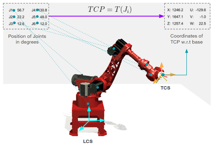
The TCP has 6 coordinates: 3 of them describes its position(XYZ) in space and the other 3 describes its orientation(UVW). The position of the joints axes and the position of the TCP is related to each other. The process of finding position and orientation of TCP given Joints values is called Forward or Direct Kinematics. Vice versa, finding our Joints values corresponding to a given TCP position and orientation is called Inverse Kinematics.

2. Coordinate Frames and Vectors

A key requirement in robotics programming is keeping track of the positions and velocities of objects in space. A frame which is essentially a coordinate system with a specific orientation and position. For example, consider the situation whereby we ask a robot to detecta blue ball in a room. It will be futile if the robot report to us that the blue is 1m from the robot because now we want to know where in the room is that blue ball. Providing this information requires us to know each of the following:

The position of the blue ball relative to the camera.
The position and orientation of the camera relative to the base of the robot.
The position of the robot in the room.

2.1 Geometrical frameworks

We need to develop a framework for representing these relative locations and using that information to translate coordinates from one frame of reference to another. In robotics, we have 4 main geometrical frameworks:

1. Global Coordinate System(GCS)

The Global Coordinate System defines the origin and orientation of our world. If our workspace consists of various robots then it is useful to define a unique global reference system so that everyone understands that same global coordinate.

The World coordinate frame is indicated with the subscript w. This coordinate frame is fixed at a known location in space and assumed not to move over time.

Fig. Global Coordinate System(GCS) in green.

2. Machine Coordinate System(MCS)

In a workspace with several robots each machine will have its own local coordinate system(LCS or MCS) which is fundamental in programming each individual robot. However, the other robots will not understand and interact with a point specified in a machine's local coordinate system. If we have only one robot then; LCS = GCS.

The machine coordinate frame is indicated with the subscript r. We can envision this coordinate frame as being attached to the base of the robot so that the origin of the frame moves as the robot moves. In other words, the robot is always located at (0, 0, 0) in its own coordinate frame.

Fig. Local Coordinate System(LCS) of each robot in blue and GCS in green.

3. Tool Coordinate System(TCS)

The origin of the Tool Coordinate System is located at the TCP of the robot. If we have no tool attached to the robot, then the TCS is at the Mounting Point(MP) of the robot.

Fig. Tool Coordinate System(TCS) in yellow and GCS in green.

4. Workpiece Coordinate System(WCS)

The most important frame for the operator in the Workpiece Coordinate System or Product Coordinate System. This frame is what the operator's sees and considers as the origin of its workplace and all the programmed points and movements refer to this system. We may have several products with which the robot will interact, hence we will have several WCS with their own origin and orientation.

Fig. TCS in yellow, GCS in green, LCS in blue and Workpiece Coordinate System(WCS) in pink.

Our goal is to understand how to move from one frame to another and how to transform coordinate points across different frames.

2.2 Frame Operations

Before we dive into frame operations, it is best we establish some conventions that we will use throughout the project. We have a left-handed coordinate system and a right-handed coordinate system. In a right-handed coordinate system we determine the direction of the z-axis by aiming the pointer finger of the right hand along the positive x-axis and curling our palm toward the positive y-axis. The thumb will then point in the direction of positive z-axis as shown below. Note that there is no way to rotate these two coordinate systems so that they align. They represent two incompatible ways of representing three-dimensional coordinates. This means that whenever we provide coordinates in three dimensions we must specify whether we are using a left-handed or right-handed system.

Fig. Left and right-handed coordinate systems and Right-hand rule for determining the direction of positive rotations around an axis.

We also need to establish a convention for describing the direction of a rotation. Again, we will follow a right-hand rule. To determine the direction of positive rotation around a particular axis we point the thumb of the right hand along the axis in question. The fingers will then curl around the axis in the direction of positive rotation.

The position and orientation of an object in space is referred to as its pose. Any description of an object's pose must always be made in relation to some to some coordinate frame. It is possible to translate a point between any two coordinate frames. For example, given the coordinates of the blue ball in the camera coordinate frame, we can determine its coordinates in the robot coordinate frame, and then in the room coordinate frame. In order to accomplish this we need to specify how poses are represented.

Suppose we have a point p in space and we have two different observers based in frame $\mathbb{F}_{1}$ and $\mathbb{F}_{2}$ respectively. Both observers are looking at point p and the first observer will record the coordinates of the point according to its frame as $p_{1}$ and consecutively the second observer records point p as $p_{2}$ . Now, the question is if we know the coordinate of point p in the frame $F_{1}$ then how do we find the position of that point from the perspective of frame $\mathbb{F}_{2}$ . If we want to convert $p_{1}$ to $p_{2}$ then we need to know how the frames $\mathbb{F}_{1}$ and $\mathbb{F}_{2}$ are related to each other. As such, the three frame operations are:

Translation
Rotation
Translation + Rotation

2.2.1 Translation

Suppose we are based in frame $\mathbb{F}_{1}$ and we observe our point p with coordinates $(x_{}, y_{}, z_{})$ . Its position from this perspective is $p_{1}$ with coordinates $(x_{1}, y_{1}, z_{1})$ . We then move our based to a new frame $\mathbb{F}_{2}$ which is translated by an offset $\Delta f$ . That same point p when observed from that new frame $\mathbb{F}_{2}$ has a new position called $p_{2}$ with coordinates $(x_{2}, y_{2}, z_{2})$ . Translation is a linear operation therefore, when coordinate frames are separated by a pure translation transforming points between frames is straightforward: we only need to add or subtract the three coordinate offsets.Hence, the new position of p is simply:

$p_{2} = \Delta f + p_{1}$

Breaking up for each coordinates, we get:

$\begin{pmatrix} x_{2}\\ y_{2}\\z_{2}\\\end{pmatrix} = \begin{pmatrix} x_{1}\\ y_{1}\\z_{1}\\\end{pmatrix}+\begin{pmatrix} \Delta x_{}\\ \Delta y_{}\\\Delta z_{}\\\end{pmatrix}$

The offset $\Delta f$ expresses how the old frame $\mathbb{F}_{1}$ is seen from the new frame $\mathbb{F}_{2}$ . In the example below, we have a negative offset along the y-axis.

2.2.2 Rotation

Specifying orientation in three dimensions is more complicated than specifying position. There are several approaches, each with its own strengths and weaknesses.

Euler Angles

In Euler angles orientation is expressed as a sequence of three rotations around the three coordinate axes. These three rotations are traditionally referred to as roll, pitch and yaw. When working with Euler angles it is necessary to specify the order that the rotations will be applied: a 90o rotation around the x-axis followed by a 90o rotation around the y-axis does not result in the same orientaion as the same rotations applied in the opposite order. There are, in fact, twelve valid rotation orderings: xyz, yzx, zxy, xzy, zyx, yxz, zxz, xyx, yzy, zyz, xzx, and yxy.

As convention, each rotation is performed around the axes of a coordinate frame aligned with the earlier rotations which is referred as relative or intrinsic rotations.

Rotation Matrix

To find out how the position of our p changes when rotating our base frame, we need to pre-multiply the position coordinates with a rotation matrix. The content of the matrix depends around which axis we rotate and the angle of rotation $\Theta$ . Below shows the rotation matrices when rotating around each individual axes:

X-axis:

Y-axis:

Z-axis:

In all cases, when the angle of rotation is 0 degrees, the rotation matrix reduces to the Identity matrix. That is the diagonal of the matrix becomes one and the rest becomes zero and that is the reason we have cosine along the diagonal and sines outside of it.

Furthermore, when we tranpose the rotation matrix we find the same matrix but with an opposite rotation angle, i.e, the rotation in the opposite angle.

It is possible to represent any orienation as a product of three rotation matrices around the x, y and z axes. It is straightforward to convert from an Euler angle representation to the corresponding rotation matrix. For Euler angles represented using relative rotations, the order is reversed.That is, a 45° roration about the x-axis, followed by 30° about the -axis and a 75° about the z-axis is represented as $R_{relative} = R_{z}(75^{\circ }) \cdot R_{z}(30^{\circ })\cdot R_{z}(45^{\circ })$

In general, rotation of robots are usually given in A,B and C angles arounf the X,Y and Z coordinate system. That is we first rotate of an angle A around the x-axis, then an angle B about the y-axis and finally an angle C about the z-axis. The notation is referred as Improper Euler angles, or RPY angles or Cardan angles.

Two important properties of rotation matrices are that:

Any orientation can be achieved composing Euler angles which is relatively easy to perform.
Any rotation matrix can be decomposed in Euler angles although that is is not that straightforward.

The rotation matrix then becomes:

Note that when decomposing that matrix to find the angle A,B and C we can get two results for an angle. That is, we can reach the same global rotation with different individual rotations around the base axes. Euler angles are not unique! Combined with the choice of axis orderings, there are 24 possible conventions for specifying Euler angles.

When $B = \pm 90^{\circ }$ , . The matrix is simplied but now A and C are no longer linearly independent. We are facing a singularity which is a partivcular configuration whreby an infinite number of solutions exist. We can only compute the sum and difference of A and C but not their individual values.

Some important properties of the rotation matrix:

The rotation matrix is an orthogonal matrix, i.e, its transpose is equal to its inverse. This is important for us and calculating the inverse of the matrix can be difficult whereas transposing it is eaxy and quick.

$R^{T} = R^{-1}$

The determinant of the matrix is equal to 1, a property which is useful when checking if the rotation matrix has the correct input. If the determinant is not 1 then it is not a correct rotational matrix however, that does not mean that any matrix with determinant 1 is a rotational matrix.

The product of the matrixes are associative but not commutative. This means that rotating about x first and then z is not the same thing as rotating about z first and then x.

To sum up:

Euler angles are relatively easy to visualize, but they are inconvenient to work with from a mathematical point of view. The key problem is that the mapping from spatial orientations to Euler angles is discontinuous: small changes in orientation may cause big jumps in the required representation. This can cause difficulties when we need to smoothly update the orientation of a moving object over time. A possible solution to this would be to use Quaternions. As a general rule in robotics, we use Euler angles only for the interface of the operator(Visualization) but we use Quaternions for all internal calculations(Interpolation).

2.2.3 Translation + Rotation(Homogeneous Transformation)

Now we need to put translation and rotation together into an individual transformation. The Homogeneous transformation matrix T, combines the rotation matrix R, for example around the Z-axis, but can be any generic rotation around the XYZ frame, and then the translational offset Δ, which can also be any generic translation along the XYZ frame. The combination of the two is a 4x4 matrix, filled with zeros under the rotation matrix and with a 1 under the translational offset. Combining the two operations together means that with a single matrix multiplication we can perform both translation and rotation of our frame at the same time.

It is important to remember that the order is not commutative: we first rotate, and then translate. If we would first translate and then rotate, the result would be totally different.

If we have a point $p_{0}$ in one frame and want to find out its coordinates as seen from a different frame, we simply pre-multiply by the homogenous matrix. Note that because the matrix is a 4x4 and the point only has three coordinates, we need to pad its vector with a 1 at the end. The final expression for $p_{1}$ looks like that. If we only have a translation and no rotation, the cosine elements along the diagonal of the rotation part will all be 1s and the elements outside the diagonal will be 0s, so that we fall back to a simple linear offset addition for the translational effects. Similarly, if the translation offset is zero, then we only have the rotation elements left.

Example:

Imagine we have a very simple mechanical structure with only one rotating axis. Note that the position of the TCP indicated by the white dot keeps changing following the rotating axis. Now we want to find the position of the TCP in the fixed robot base frame. For that we need some geometrical parameters: the length of the arm l, and its height h. The position of the TCP as seen from the mobile frame of the robot’s moving link is actually constant. We call it $p_{0}$ with coordinates $\begin{bmatrix} l& 0& 0& 1\\\end{bmatrix}^{T}$ .

Now, to find out $p_{1}$ from $p_{0}$ , we need to find out what transformation modifies the old mobile frame into the new fixed frame at the base. We first have a rotation by an angle θ around the Z-axis, and then a translation of h along Z. Note that both are positive as seen from the new frame. So we can write down the homogenous transformation using an offset h along the Z-axis and a rotation θ around the same Z axis. h is always constant, but the angle θ can change all the time because it is driven by the rotating axis. So we pre-multiply $p_{0}$ by the matrix T to find $p_{1}$ .

To sum up:

If we have the position of a point given in one frame and want to find its position from a different frame we need to apply some transformations.
The first and simplest is a linear translation, which mathematically is a simple additionof an offset.
If the frames are rotated with respect to each other, we need to use a rotation matrix, which is built as a combination of rotations around individual axes.
Finally, if both translation and rotations are present, we can use a homogeneous matrix, which combines both operations into a single one.

3. Forward Kinematics

After studying frame operations, we can now build a geometrical model that will allow us to calculate the position and orientation of each link. This model is knows as a Kinematic model. There are two types of kinematic model: forward transformation(or Direct transformation) and inverse transformation.

Forward kinematics is defined as the process of calculating the position and orientation of the TCP given the current values of the joint axes. We know the position of the joints from the values obtained from the encoders of the electric servo motors. Using these values, we need to calculate the position XYZ and orientation UVW of the TCP always w.r.t the base frame. This function is a simple transformation between the base frame and the TCP frame.

The final transformation matrix is a homogeneous transformation that depends on all the joints positions and mechanical parameters of the robot. What we do is simply compose a chain of frames translations and rotations from the base to the TCP.

The final point $p_{1}$ can be expressed in the base frame as its local coordinates $p_{0}$ pre-multiplied by the homogeneous frame transformation. Note that now all those frames can rotate and translate with respect to each other, according to the joints values, so their angles are not constant, but parameterized.

So what are these parameters of our kinematic model? That is, what translations and rotations we observe between the different frames?

we have all the rotations introduces by the movements of the joints: from joint 1 to 6. These are not constant in time and change accordingly to the motors’ movements.
we have all the translational effects due to the mechanical size of the arm. The distance from each joint to the next as shown in the picture above, from the base to the first joint, all the way to the last one. Unlike the rotational parameters, the translational parameters are actually constant, because the mechanical size of the arm does not change in time.

3.1 Forward Kinematics: Base to TCP

We will now build our kinematic model step by step from the base to the TCP.

3.1.1 Base to J1

We have a translation and a rotation along the Z-axis. The homogeneous transformation, $T_{1}$ , for this first step is built from the rotation matrix $R_{1}$ and the offset .

Translation:

Rotation J1 around Z:

Homogeneous Equation:

3.1.2 J1 to J2

The second step goes from the first to the second joint. Here we have two translations, one along X and one along Z. Plus the rotation of the second joint around the Y axis. We build the homogeneous transformation matrix $T_{2}$ accordingly.

Translation:

Rotation J2 around Y:

Homogeneous Equation:

3.1.3 J2 to J3

From J2 to J3 we have a vertical translation along the Z axis: a3z. This is usually the longest and heaviest arm of the robot and the motor at joint 2 needs to be quite large. We build the homogeneous transformation matrix $T_{3}$ using the translation along the Z-axis and then the rotation around the Y-axis.

Translation:

Rotation J3 around Y:

Homogeneous Equation:

3.1.4 J3 to J4

The actual mechanical configuration can change according to the robot we are working on. Here, we have only two offsets, one along Z and another one along X. In other robots, there might also be one offset along Y. The homogeneous equation is build using the translation a4x and a4z and the rotation matrix about X.

Translation:

Rotation J4 around X:

Homogeneous Equation:

3.1.5 J4 to J5

With the next step we reach the middle of the wrist called the wrist center point. We simply add a translation along the X axis and a rotation around Y.

Translation:

Rotation J5 around Y:

Homogeneous Equation:

3.1.6 J5 to J6

We finally reach the end of the robot with the last step: one additional translation and rotation along X.

Translation:

Rotation J6 around X:

Homogeneous Equation:

3.1.7 Base to J6

The XYZ coordinates of the TCP as seen from the base frame can be obtained by pre-multiplying the position of the TCP in its local frame, which is zero, the origin of the TCP frame, by all the homogeneous transformations(T1 to T6) we obtained for each frame in the previous six steps. The advantage of this solution is that it can be applied to any open kinematic chain.

For the rotation coordinates ABC of the TCP we do the same thing, using the rotation matrices we built in the previous steps. Since the product is associative, we can split the calculations in two:

The first, second and third joints determine the rotation of the arm, from the base to the wrist center point.
Then the fourth, fifth and sixth joints determine the rotation of the wrist from the wrist center point to the TCP.

Position:

Rotation:

3.1.8 GCS to Base to J6

So far we have calculated the position and orientation of the TCP as seen from the local robot’s frame or Machine Coordinate System(MCS). Now we want to know the position of the TCP in the Global Coordinate System(GCS) so that other robots can also work with it.

For the position, we need to pre-multiply by the homogeneous matrix that describes the transformation between local machine coordinate(MCS) system and global world coordinate system(GCS).

For the orientation, it is enough to pre-multiply by the rotation matrix.

3.1.9 Base to J6 to TCP

Now if the TCP is not the mounting point but instead we have a tool at the end of our MP then we need to add the homogeneous matrix and the rotation matrix after the multiplication chain.

Position:

Rotation:

3.2 Mechanical Coupling

In practical, there are axes of the robot that are internally mechanically coupled. For example, a movement of J5 causes a movement of the J6 even if the motor of J6 is not moving. Hence, we need to compensate for this effect in our calculation.

In the picture below, only J1 is moved and J2 is remained fixed. However, due to the mechanical coupling, J2 is forced to move even if the motor was not activated. The white dotted lines shows the difference between the actual positions reached by the arm with and without mechanical coupling. That difference is a function of the coupling coefficient between J1 and J2.

We normally solve the direct transformations between joints and TCP with the forward kinematic function. But the joints positions are what we read from the encoders, they do not represent the actual position of the joints angles if an additional mechanical coupling is present.

For our 6-axis robot, we introduce coupling coefficients in the forward kinematic model so that the actual position of the TCP is calculated correctly. Before we send those joints values from the encoders to the forward kinematics, we need to adjust them by the coupling coefficient: for example the actual position of J5 and J6 might be influenced by the position of the J4. In that case the final value is what the motor sees plus the coupling factor function of J4.

4. Inverse Kinematics

Up until now, we have studied forward kinematic whereby we are given the joint angles(J1 to J6) of the axes and we need to calculate the position and orientation of the TCP or End-Effector. We showed how we could use the Homogeneous transformation matrix H, to find the location of our end-effector.

In inverse kinematics we are given the TCP location and we are asked to find the joints angles(J1 to J6) that result in that particular TCP location. Inverse kinematics is more useful for us as this is the kind of situation that we will be dealing with in real-world. That is, we may know a particular object location that our end-effector will need to grab and we will then need to find out the desired joints angles of our robots to achieve this task of grabbing the object. Remember that the TCP coordinates are expressed relative to the base frame.

Robots are programmed by the operator in path space coordinates (XYZ), which are clearly understood. But motion control software acts directly on the motors, which move the joints of robots. So we need a way to transform back from path space to the joints space. More explanation about these two spaces are found below:

An industrial robot can be controlled in two spaces: Joints space and Cartesian space. Hence, there are two sets of position-mode motion commands that make an industrial robot move. For joint-space motion commands (sometimes incorrectly called point-to-point commands), you simply specify — directly or indirectly — a desired set of joint positions, and the robot moves by translating or rotating each joint to the desired joint position, simultaneously and in a linear fashion. For Cartesian-space motion commands, you specify a desired pose for the end-effector AND a desired Cartesian path (linear or circular). To find the necessary joint positions along the desired Cartesian path, the robot controller must calculate the inverse position and velocity kinematics of the robot. Singularities arise when this calculation fails (for example, when you have division by zero) and must therefore be avoided.

Try jogging a six-axis robot arm in Joint space, and the only time the robot will stop is when a joint hits a limit or when there is a mechanical interference. In contrast, try jogging the same robot in Cartesian space and the robot will frequently stop and refuse to go in certain directions, although it seems to be far from what you think is the workspace boundary. A robot singularity is a configuration in which the robot end-effector becomes blocked in certain directions.

Unfortunately, the inverse kinematics problem is so hard that sometimes it is even impossible to solve the problem in closed-form, that is we cannot write down equations to derive the joints axes values and a numerical approach is required. In other times, we will need a couple of assumptions and even geometrical intuition in order to solve the inverse kinematics.

For a 6-axes robot the condition that allows for a closed-form solution is the configuration of the wrist. We have two kinds of wrists: spherical and non-spherical wrist robots.

4.1 Spherical wrist robot

In the spherical wrist, the three rotating axes J4,J5,J6 all intersect at one point at the wrist center point. This configuration is the most common in the industry and allows for a nice closed-form solution.

4.2 Non-spherical wrist robot

In the non-spherical wrist, the rotation axes do not intersect at one point. This configuration requires a numerical solution(trial-and-error procedures - approximation to the solution of a mathematical equation) so it is mathematically more complex and computationally more expensive. However, it does not suffer from singularity issues and can always perform movements at constant speed. For that reason it is used often in painting applications, where a constant speed is strictly required to spray a uniform layer of paint.

4.3 Non-unique solutions

Another problem that makes solving inverse kinematics complicated, is the fact that, given a particular target position and orientation of the TCP, there might be more than one way for the joint axes to configure in order to reach that pose. In other words, the solution to the inverse kinematics is not always unique!

4.3.1 Non-unique solution I: Up and Down

In this example we have a target position which is same for both robot. Both robots reached the same target with two different configurations. Observe that the TCP position and orientation are absolutely the same in both cases. But the joint axes configurations are different!

We call the two options UP and DOWN. This is also a problem for the operator while programming the robot. In our software interface we need to provide a way for the operator to choose the preferred option, either up or down, or maybe we can automatically select the solution closest to the current joints configuration.

4.3.2 Non-unique solution II: Front and Back

The next example is even more extreme. We move the two robots to the same target TCP pose and we notice how they select completely different solutions whereby the second motion is absolutely redundant and overly complex.

The main difference here is J1, which can either point in the front or the back of the robot, hence, the name FRONT and BACK.

4.3.3 Non-unique solution III: Positive and Negative

The next example is more subtle. The final configurations look the same but they are not. While J1, J2 and J3 are in the same position and give the same pose to the arm, the last three joints are in different positions and give a different configuration to the wrist. Notice that the J5 has opposite values in the two cases, hence, we call one POSITIVE and the other NEGATIVE.

In all these previous examples we were able to find two distinct solutions to the inverse kinematics problem.

4.4 Singularities

Now, we will see that there are cases where an infinite number of solutions are available. These critical points are called singularities, and occur for some specific target poses of the TCP. There are 3 types of singularities: Shoulder Singularity, Wrist Singularity and Elbow Singularity.

4.4.1 Shoulder Singularity

In the shoulder singularity, the wrist center point from J4, J5 and J6 aligns with the center point of J1. If we try to move from this position we will notice that the J1 and J6 will start to rotate very fast in opposite direction. The TCP will remain almost still causing a very inefficient robot motion. We can find a fixed solution for most joints, except for J1 and J6. These two are linearly dependent and we can only find their sum or difference. Therefore, an infinite number of possible solutions are available.

Recall that a matrix is singular when its determinant is zero. The associated linear system has an infinite number of solutions because two or more variables are dependent on each other.

4.4.2 Wrist Singularity

In the wrist singularity, J5 is 0, while J4 and J6 are not independent anymore. We can move them around without modifying the final pose of the TCP. We have an infinite number of solutions. Normally, we manually pick a value for one of the two joints, for example J4, and then the other joint is automatically fixed.

4.4.3 Elbow Singularity

Imn the elbow singularity, J2, J3 and the wrist center point aligns together. When these 3 points are aligned, the elbow of the robotics arm will get stuck in the so called elbow singularity no matter where the TCP is. Elbow singularities look like the robot has “reached too far”, causing the elbow to lock in position.

To sum up:

the inverse kinematic problem is more complex than forward kinematics, not only because it is difficult to find a solution, but because sometimes there are many, or even infinite possible solutions we need to pick from.
the definition of singularity is when the robot has an infinite number of kinematic possibilities to reach the same end position - an infinite number of ways to get to the same spot.
what a robot's kinetic algorithm is trying to do is solve a complex equation of where to put all our axes(J1 to J6) to get our tool where we need it to be. The operator will just drag this robot somewhere and say record and we just take for granted that it gets there. But if there are an infinite number of solutions to get there then it does not know which one to take hence, we find singularity and the robot faults out.

Below is a video showing the singularities explained above:

Y2Mate.is.-.What.are.robot.singularities-lD2HQcxeNoA-480p-1641578742646.mp4

[Video by Mecademic Robotics](https://www.youtube.com/watch?v=lD2HQcxeNoA)

4.4.4 Avoiding Singularities

It is kind of hard to tell you where we are likely to find the most singularities since they are not at a given position, they are relative to the robot configuration. In simpler words, singularities occur when a robot loses a degree of freedom.

There are two ways we can find these singularities:

- Inspection: Here we just observe and determine what would be a singulafrity for that robot.

- Calculation: We write the Forward Kinematic equations, take the derivative of the velocity, find the Jacobian matrix and set its determinant equal to zero to find the joints angles that would make the determinant = 0.

Singularities most occur in nature when we place objects to be grabbed by the TCP at right angles and having the object below at the base of the robot. The image below shows that J5 is 2 degrees away from zero. The table is too low and the object is too close to the base of the robot. The robot would go pick the object but if we go a little bit back then we hit a singularity. There are many places singularities can occur becasue anytime J5 is 0 I can hit a singularity. One important thing to remember is that when in a situation as depicted in the image below, the programmer is powerless. There is nothing robotics programmers can do as they are bounded by unsolvable mathematical equations. However, we can redesign the workplace to avoid such occurances as explain below.

Below are 6 ways to avoid singularities:

1. Choose another robot: We can only get a singularity with a 6-axis or more robot. If we have a four axis robot, there is no such thing as singularity. It cannot happen because any place we want to go there are no two axes fighting each other hence, we have only one solution.

2. Singularity Avoidance package: This is a package when buying a robot that imbed some built-in intelligence to the robot to avoid these singularities. It's going to make movements that will result in only one solution.

3. Re-design workplace: We could relocate the robot by lowering it relative to the picking surface or change the table's postion, i.e, we increased the height and placed it a bit further from the base and this result in a change in the articulation of the robot arm. We now have a nice bend between J4 and J5(57.6°).

4. Offsetting the tool: By offsetting the tool as shown below, we force the robot to be further away from the object. In that way we induce a small angle(about 15 degrees) whereby we used to have only about a 2 degrees angle. Offsetting the bracker allows us to gain some reach - our J6 can not swing - and it also allow us to manipulate the tool as per our needs.

5. Pivot the tool: We can also pivot our tool such that when picking the object, the tool is perpendicular to the object but we have about 30 degrees angle at our J5. We are far away from zero therefore far away from a singularity.

6. Tilt robot: The next solution would be to tilt the robot - about 30 degrees - such that the robot is fixed on a wedge block and we have a nice J4 and J5 interaction with a bend of 24 degrees.

To sum up:

it is mostly the mechanical engineer work to find a suitable solution for the robot to avoid singularities. The programmer should already plan this on his software.
it is important to plan ahead of the position of the robot or workbench or tool so as to avoid redundant changes in the physcial robot.
robot singularities can only be avoided by properly designing our robotic cell (and that includes the design of the adaptor plate for our end-effector).

4.5 Inverse Kinematics: Arm

Earlier we discussed that our robot is a spherical wrist robot as J4,J5 and J6 all intersect at the wrist center point(WP). That point is crucial because it is dependent only on J1, J2 and J3. That is, only a movement of J1, J2 and J3 can change the position of WP and not J4, J5 and J6. Hence, we can split the robot into two parts: arm and wrist. We will process as follows:

Given the position of the WP, we can find J1, J2 and J3.
Then gicen the position and orientation of the TCP, we find J4, J5 and J6.

This process is called decoupling, i.e, we decouple the wrist from the arm and this process is only possible for spherical wrist and J4, J5 and J6 do not affect the position of WP.

4.5.1 Finding WP

We have shown before that the difference between WP and TCP is a6x which is the offset between J5 and J6. However, this offset runs along the x-axis of the local TCP frame, which we call $\hat{x}$ in the robot’s base frame.

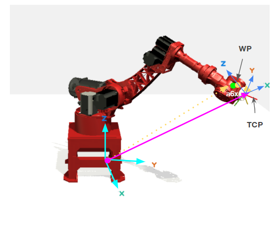
Given the orientation of the TCP in Euler angles, we know how to compose the equivalent rotation matrix by multiplying together all the individual rotations around the XYZ axes.

We then take the rotation matrix R, multiply it for the local x vector $\begin{bmatrix} 1& 0& 0\\\end{bmatrix}^{T}$ and we find how this vector is seen from the base.

From the multiplication above, we get the first column of R, which is $\hat{x}$ . We subtract a6x times $\hat{x}$ from the TCP position to find out the WP position.

After finding WP, we can now find J1, J2 and J3.

4.5.2 Finding J1

The position of J1 only affects the X( $WP_{x}$ ) and Y( $WP_{y}$ ) coordinates of the wrist point, not the vertical position Z( $WP_{Z}$ ). So we can reduce the problem to a 2-dimensional planar problem and observe that J1 is the angle between the X and Y coordinates of WP. The solution is simply to take the arctangent.

Recall that two solutions are possible for this problem, depending on the pose that we select: either front or back. In the first case J1 is what the arctangent function returns; in the second case we need to add 180 degrees.

Finally, if both X and Y are zero, the wrist point is straight above the base origin and we have a shoulder singularity. Any position for J1 would be a correct solution. We usually fix J1 equal to the actual position of the joint.

4.5.3 Finding J2 and J3

When J1 is fixed, movements of J2 and J3 only happen on a vertical plane. So we can simplify the problem by removing one dimension and reduce the workspace to a 2D geometry as shown below. We need to focus on the green triangle to find J2 and J3.

First using pythagoras theorem, we unified the X and Y coordinates into a single XY( $WP_{xy}$ ) component.
We will focus on the green traingle to solve for J2 and J3. One of its side is $\rho$ and its horizontal and vertical projections are h and l respectively. Since we know the mechanical size of the robot we can easily find h and l. We then using pythagoras theroem to find $\rho$ .
We already know another side of the green triangle: a3z. We know need the last side which is b4z. We observe that it is the hypothenus of the yellow triangle on top with legs a4z and a4x+a5x.
In order to avoid a situation whereby the robotic arm tries to reach an object toor far from the TCP, we need to apply the triangle inequality. We limit the value of $\rho$ using this rule.

The sum of the lengths of any two sides of a triangle has to be greater than the length of the third side and the difference of the lengths of any two sides of a triangle has to be less than the length of the third side.

Now we need to find $\alpha$ using the arctan of h and l.
We find $\beta$ using the cosine rule.
We observe that J2 + $\alpha$ + $\beta$ = 90°. We solve for J2. Note that it could also be plus $\beta$ , if we were to choose the DOWN pose instead, with the second link pointing downwards and the third upwards.
We find $\delta$ using arctan.
For the top yellow traingle, we observe that J3 + $\gamma$ + $\delta$ is 180°. We solve for J3.

4.6 Inverse Kinematics: Wrist

The first three joints(J1, J2 and J3) determine the position of the wrist point and also the orientation of the arm from the base up to the wrist center. We call that rotation matrix $R_{arm}$ The rotation of the TCP is given by the matrix R, which we already found composing the ABC Euler angles. The missing rotation in between those two is given by the $R_{wrist}$ matrix.

R is the product of $R_{arm}$ times $R_{wrist}$ , we can solve for $R_{wrist}$ pre-multiplying both sides by $R_{arm}^{-1}$ and simplifying the right side. $R_{wrist}$ is then the product between $R_{arm}$ transpose and R.
Since $R_{arm}$ is an orthogonal matrix, we know that its inverse is equal to its transpose.
Remember that is $R_{arm}$ the rotation matrix from the base to the frame created by J1, J2 and J3. Hence, we need to compose the rotations of the joint J1 around the Z-axis, and of J2 and J3 around the Y-axis.
The R matrix is found from A,B,C hence we can now derive $R_{wrist}$ .
After finding $R_{wrist}$ , we need to decompose it into its individual rotations of J4, J5 and J6. Remember that J4 rotates around X, J5 around Y and J6 around X again.
We then need to decompose the $R_{wrist}$ matrix into Euler angles to find J4, J5 and J6.
However, if cosJ5 = 1 then J5 = 0. We will then have a wrist singularity. There is no rotation around the Y-axis, only two consecutive rotations around X. There is no way to separate J4 and J6 anymore. Only the sum of their values is known, because it is essentially a single rotation about the X-axis. The $R_{wrist}$ ,matrix then becomes:

The solution is to fix one of the two angles, for example J4 equal to its current value, and find J6 accordingly.
We always try to minimize the robot’s movement’s distances to reach a target position. Hence, since angles are periodic we can add or subtract $2\pi$ to get the most convenient solution.

We must remember to adjust for our coupling joints. The output of the inverse kinematics model is the positipm of the real joints. They must be adjusted to calculate the correct motor target positions.

To sum up:

Manipulator tasks are normally formulated in terms of the desired position and orientation.
A systematic closed-form solution applicable to robots in general is not available.
Unique solutions are rare, multiple solutions do exist.
Inverse kinematics: Given a desired posiion X,Y,Z and orientation A,B,C, we find values of J1,J2,J3,J4,J5 and J6.

5. Path Planning

In path planning, we will study the geometrical description of the robot’s movement in space. The geometrical curve to move between points is what we call the path. If we have to points in space - A and B - we can have several ways to travel from A to B. We can have the shortest route which is the displacement - a straight line from A to B or we could have some random curve path joining the two points. Once we fix the geometry we want, we also need to generate a time-dependent trajectory to cover the path.

The easiest way to move from one point to another one, is by simply moving the joints axes of the robot to their target positions. This is called point-to-point(PTP) movement. PTPs are fast but they do not provide any specific control over the geometrical path of the TCP.
If we want control over the geometry of the path, then we need an interpolated movement, for example a line. Other interpolated movements are the circle, and the spline which is a smooth interpolation through some target points in space.

5.1 Point-to-point(PTP)

Point-to-point is a linear interpolations of the joint axes of the robot. How does it work? Suppose we start from point $p_{0}$ , where all the joints have certain values and we want to reach point $p_{1}$ , where the joints have different values. We simply linearly increase or decrease the joint angles, from their starting to their target values.

We use the parameter t to describe the equation of this movement.
t = 0 at the starting point and t = 1 at the end of the movement.
If we pick any value between 0 and 1, the joint axes have a value of $p = p_{0}(1-t)+p_{1}t$ .
when t = 0, $p=p_{0}$ and when t = 1, $p=p_{1}$ .

Note:

t is not time. t is just a parameter describing the curve from 0 to 1. It describes the path but not the trajectory. Here, we only plan the geometry, not the speed of the movement. So no time is involved.
This linear interpolation happens in the Joint space. The joint angles move linearly from their starting position to their target value. For example, joint J1 could move from 0 to 80 degrees. However, this linear movement of the joints does not translate at all into a linear movement of the TCP. If we imagine the first joint moving from 0 to 80 degrees: the TCP actually moves around a circle in space(remember that J1 is a rotation around the Z-axis.)!
While PTP movements are very simple to program and fast to execute, they also have no control over the actual path of the end effector of the robot. At planning time we do not know what the position and orientation of the TCP will look like.

Although the TCP movement is not a line, the formula we need to calculate this movement is a linear interpolation between $p_{0}$ and $p_{1}$ . As t increases, $p\mapsto p_{1}$ . As shown from the graphs above, the value of J1 changes linearly as t increases.

5.1.1 Point-to-point(PTP) vs Path Interpolated

If we want to reconfigure the arm, e.g. change from UP to DOWN, the only way we can do that is with a PTP movement, where the joint axes are free to move independently from each other to their final target value.
A path-interpolated movement does not allow that. If we start a line in space with an UP configuration we will arrive at the end of the line with the same UP configuration. That is because the geometry of the arm is restricted during path movements. It cannot stretch and reconfigure itself in a different way without sending the TCP out of its planned path.
PTP movements, on the other hand, do not care about the TCP path and can essentially do whatever they want to the geometry of the links.

To sum up, PTP movements are time-optimal, that is, they always take the shortest time possible to complete from start to end. Finally, and most importantly, a PTP movement is the only movement that allows a modification of the actual joint configuration.

5.2 Path Interpolation

In order to describe a target pose for our TCP in space, we need 6 coordinates hence, the reason for our robot to be a 6dof robot. Suppose we have a starting point $p_{0}$ with coordinates XYZ and we need to move to our next position $p_{1}$ with coordinates X'Y'Z'. This time we are expressing the joints in the Path space instead of the Joint space. Moving from one point to the next can be done linearly, i.e, one unit top and one unit to the right. And to return back we have two options; either one unit down and one unit left or one unit left and then one unit down. Either way we will return to our starting position! This is because we are working in a Euclidean space, where vectors add up linearly. The process can be seen below:

However, this is not the case for our TCP angles UVW because Euler angles do not interpolate linearly. This happens because Euler angles do suffer from Gimbal lock where the order in which we apply the three rotations affects later rotations in the sequence. Below shows the process of first rotating around X of 90 degrees, then rotate around Z also of 90 degrees to reach $p_{1}$ . And then we go back, X of -90 and Z of -90. If rotations did add up linearly like positions we would go back to the initial pose but this not what happened!

A better way to interpolate these orientations is to convert our Euler angles into another representation before interpolating them. Rotation matrices is one solution but matrices are not suitable for interpolations as they cannot be parameterized with one single variable running from 0 to 1. A better solution would be to use Quaternions.

5.3 Quaternions

Since Euler angles suffer from singularities at 90 degrees, we need another way in order to interpolate angles: Quaternions. The general expression for quaternion is:

where is a vector and w is a scalar. i,j and k are complex numbers hence:

The 4 elements x,y,z,w define the quaternion and are the number of elements it needs to describe an orientation, as opposed to 3 elements for Euler angles and 9 for a rotation matrix. We typically work with unit quaternions: that means a normalized form, where the norm of the quaternion is simply the Euclidean size of the vector of elements x,y,z,w.

where ${\left\| q\right\|} = \sqrt{x^{2}+y^{2}+z^{2}+w^{2}}$ .

Suppose we have a vector v in 3-dimensional space and we want to rotate it about point p at an angle $\theta$ .

We will use quaternion to rotate it and we start by defining our quaternion and its complement:

If we are rotating at an angle of $\theta$ , then a,b,c,d are defined as :

Any given orientation is described by one unique quaternion. That is unlike Euler angles, with which many representations were possible for the same orientation in space. After defining a,b,c,d, our corresponding unit quaternion is defined by:

If p is the point around which we are rotating, we write p as a quaternion:

And finally the rotation is :

5.3.1 Quaternions Advantages over Euler Angles

Compared to Euler angles, quaternions do not suffer from singularities: they offer a unique undisputable way to identify rotations.
They also offer an easy way to interpolate linearly between orientations.

5.3.2 Quaternions Advantages over Rotation Matrix

Quaternions are more compact: using only 4 elements instead of 9.
Matrices are also impossible to interpolate, and they are not numerically stable.
It is possible that a rotation matrix undergoes several computations and comes out non-orthogonal because of numerical approximations, that is, its determinant is not 1 anymore. In that case the matrix is very difficult to recover.

5.3.3 Spherical Linear Interpolation(Slerp)

Given two orientations, represented by the two quaternions $q_{1}$ and $q_{2}$ what is the shortest and simplest way to go from one point to the other? Since we move along a sphere, there are infinite ways to do this but we are interested in the optimal path - the torque-optimal solution which uses the minimum energy to travel from the start to the end.

The solution is defined by the formula below, which is equivalent to a linear interpolation in Euclidean space, but this time we move on a sphere. We still use the parameter t, which goes from 0 to 1.

We can travel along the rotation at constant angular speed. This kind of interpolation is called Slerp. Alpha is the angle between the two quaternions, and it is calculated the same way as the angle between vectors on plane:

Note that the problem with the arccosine is that it can return two different angles between the quaternions: either the shortest one of the opposite one. To guarantee that we always use the shortest angle we need to make sure that the dot product between the two quaternions is positive before taking the cos inverse. If we happen to have a negative dot product then we should invert it by inverting one of the two quaternions, i.e, multiple one of the quartenion by -1. We will still reach the same rotation, just using a different path.

Also, if the angle between the two orientations is very small we could face numerical instabilities with that $sin\alpha$ at the denominator. Observe that a small arc on the sphere essentially degrades into a linear segment, so we can use the standard linear interpolation instead, and have more stable calculations.

As shown below, when moving the TCP around a particular axis, only the orientation of the TCP chnages and not its position, i.e, the XYZ values remain constant.

quaternion.mp4

5.3.4 Implementation

We have the start( $A_{0}B_{0}C_{0}$ ) orientation of the robot and the user provides a target( $A_{1}B_{1}C_{1}$ ) orientation. We cannot interpolate the ABC Euler angles directly so we interpolate quaternions using Slerp.

We first transform the Euler angles into Rotation matrices and from there into Quaternions.
Then we apply SLERP to interpolate between $q_{0}$ and $q_{1}$
But because we control the motors of the robot we need to solve the inverse kinematics to find out the values of the joint axes. So we need to transform q back into a Rotation matrix and then Euler angles as input to our inverse kinematic function.

To sum up:

There are a few advantages of using quaternions over Euler angles or rotation matrices, the most important of all for our purposes being the possibility of interpolate them. When we move the robot from one pose to another we need to change its orientation from the initial one to the final one. This smooth change over time is called interpolation. We cannot interpolate matrices or Euler angles directly. Quaternions can do that easily with SLERP.

5.4 Lines

The simplest interpolation in the path space is a line. We start from point $p_{0}$ with coordinates $(x_{0},y_{0},z_{0})$ and want to reach $p_{1}$ with coordinates $(x_{1},y_{1},z_{1})$ . The formula for linear interpolations is as explained before: $p=p_{0}(1-t)+p_{1}t$ , with t going from 0 to 1.

We may have two situation in practice:

In the first case the starting and target points have the same orientations, so the interpolation only happens on the position coordinates XYZ.
In the second case the initial and final orientations are different. So, while the position coordinates interpolate linearly, the orientation interpolates using SLERP. The two interpolations happen in parallel at the same time.

5.5 Circle

Two points are not enough to define a circle in space. We need three points: the starting point $p_{0}$ , an intermediate point $p_{1}$ and the final target point $p_{2}$ . The parametric formula for the position of a point describing a circle in space is the following:

C: center point

r: radius

U: normalized vector from the center to the starting point
V: a vector perpendicular to U, lying on the circle plane
t: the parameter that runs around the circle, from zero to the ending angle

Note: We need to check the points are not collinear, i.e, no points lie on the same line in space. The vectors U and V are perpendicular to each other and form the analogue of the X, Y axes on a plane.

So starting from t = 0 we point along the vector U and we then rotate around using the formula in 2D: rcos(t) + rsin(t). This is a group of three individual equations: one in x, one in y, and one in z. We are only focusing on position here, because the orientation will follow the SLERP interpolation: from the start orientation to the middle orientation and to the ending one.

To sum up:

We need to find all the points between $p_{0}$ (where the movement starts) and $p_{2}$ (where the movement ends) along the circle.
If we take a simple 2D case - the X,Y plane - the parametric equation of a circle centered in the origin is p = r cos t + r sin t. By moving the value of t from 0 to any angle we want (positive or negative), we will find the coordinates of the point p along the circle.
If the circle is not centered in the origin, we need to add the coordinates of its center point: p = C + r cos t + r sin t.
Finally, if we move to the 3D space and the circle does not lie on the X,Y plane we need to generalize its axes to the vectors U,V. In the 2D case the U,V vectors were simply [1,0] and [0,1]. The generic formula for a circle in 3D becomes p = C + U r cos t + V r sin t. U and V are perpendicular to each other and both lie on the same plane where the circle lies.

5.6 Splines

Suppose we have a starting point and a target point and we want to join these 2 points smoothly, i.e, not with a straight line. We will then use a spline to join these 2 points. Splines are functions built up by composing polynomials piece-by-piece. In our case, we will use a Bézier Curve for the spline and to be more precise, we will use Cubic Bézier Curve.

5.6.1 Bézier Curve

Bezier Curve is parametric curve defined by a set of control points. Two points are ends(starting and ending points) of the curve. Other points determine the shape of the curve. The Bézier curve equation is defined as follows:

t: [0,1]
P(t): Any point lying on the curve
$B_{i}$ : ith control point on the Bézier Curve
n: degree of the curve
$J_{n,i}(t)$ : Blending fucntion = $C_{(n,i)}t^{i}(1-t)^{n-i}$ where $C_{(n,i)}=\frac{n!}{i!(n-i)!}$ .

The degree of the polynomial defining the curve segment is one less than the total number of control points. Since we will be using a cubic curve, our number of control points will be 4.

Substituting for n = 3 in the above equation, we get:

$B_{1}$ and $B_{2}$ are control points used to define in what direction and with what magnitude the curve moves away from the 2 edge points. We have a total of 4 control points because we decided to use a cubic spline in the parameter t where t = [0,1]. Every point P on curve is a linear combination of the four control points, with the weights being the distances from them. Note that the control points are always placed tangential to the starting and ending points respectively.

Note: A common rule of thumb is to keep the control points distance at about 1/3 of linear distance between start and end point.

Bézier curve is a valuable function for robot’s operators: they can just teach the position of some points where the robot is required to go through and we automatically generate the whole path in between. For example, if we we need to move our robot from one point to the other but we have an obstacle in between, then we just need to define a third point above the obstacle and let the algorithm calculate a smooth path between the three points as shown below:

Also, while the spline runs the position of the TCP, we can interpolate the orientation in parallel using quaternions.

5.7 Continuity and Smoothness

We have studied different geometries to connect two points in space. Now we need to study how to connect those geometries with each other. The point between two consecutive segments of a path is called a transition. The first problem we encounter when observing transitions is that there might be a sharp angle between them. These sharp edges are bad because when we travel along the path we have to decelerate, stop at the transition and then start accelerating again along the next section. This behavior not only wastes a lot of time but is also hard on the mechanics. A smoother movement would be much more desirable. One possible solution is to introduce a round edge as a path smoothing transition. You notice that the path is smoother, which allows for higher travelling speed because no stop is required, and it is also gentle on the mechanics. Hence, the reson for using a Bézier curve.

Suppose we have two perpendicular consecutive paths section then we will need a round edge for a smooth transition.

First we need to limit our radius R by setting it half the length of the segment. This is incase we have another round edge at the next transition thus, we leave some spave for that.
Once we have R, we need to define two control points: starting( $\bg_white P_{0}$ ) and ending( $\bg_white P_{4}$ ).
Instead of using a cubic spline, we will use a quartic spline hence, we have 5 control points.
We place one( $\bg_white P_{2}$ ) at the transition and the two( $P_{1} and P_{3}$ ) left are placed in middle of the other control points.
This configuration ensures geometrical continuity of the spline with the original line up to the second derivative: i.e, the two sides have same direction and also same curvature. The transition between line and round edge is smooth.

5.7.1 C0 Continuity

We need the path to be smooth but how do we define smoothness? In order to check for smoothness, we need to first ensure that our path is continuous. What is important is to find the direction of the tangents at the transition points. In general:

A function f(x) is smooth if it is continuous and its derivative is also continuous.

The figure below shows a $C^{0}$ continuous graph as we have two paths which meet at one point. The tangent of the two paths point in two different directions as shown in blue below. The edge is sharp and not smooth.

The class $C^{0}$ consists of all continuous functions.

5.7.2 C1 Continuity

In the next figure, the two curves touch at the transition point. We say we have $C^{1}$ continuity as the tangents of the curves and surfaces are vectors with both the magnitude and direction of the tangent vectors being identical.

The class $C^{1}$ consists of all differentiable functions whose derivative is continuous; such functions are called continuously differentiable. Thus, a $C^{1}$ function is exactly a function whose derivative exists and is of class $C^{0}$ .

The second derivative represents the smoothness of the curve. Although we have a transition of a circle with a line, it is not smooth, i.e, we do not have a $C^{2}$ continuity. As described above, having the same tangential direction implies only $C^{1}$ continuity, which translates into same speed of movement, but different accelerations. The fact that this transition between line and circle is not $C^{2}$ means that if we travel at constant speed across the transition, the acceleration along the vertical axis changes instantaneously: from zero along the line, to a sudden finite positive value when entering the circle. In practive we will hear a "click" sound on the axes, which can be detrimental to the mechanics.

The continuity between two curves must be satisfied at higher order of differentiation so as to have a smooth dynamic profile and avoiding slowing down or, worse, stopping the trajectory. Thus, the reacon for using $C^{2}$ continuity.

5.7.3 C2 Continuity

The figure below shows $C^{2}$ continuity as they have the same tangential direction and the same curvature.

We do not always need $C^{2}$ transition but we need to check that the transition angle between consecutive sections is small enough so as to increase production speed and to avoid excessive force on the mechanics.

5.7.4 Proving C2 Continuity

Earlier, we introduced a round-edge between two lines as a quartic spline and said that the transition is smooth up to the second derivative. Note that this round edge is not a circle! The transition between line and circle is not $C^{2}$ continuous, as we mentioned before. The circle has a constant radius of curvature, which means a constant finite second derivative. When crossing from line to circle the curvature jumps suddenly. But the round edge is a quartic spline, not a circle. Its radius of curvature is not constant: it starts at zero, increases in the middle and goes back to zero at the end, so that the transitions with the previous and next segments are smooth.

Let's prove the smoothness mathematicaly: We start with a line segment which parametric equation is as follows:

First derivative w.r.t t:

Second derivative w.r.t t:

This clearly shows that a line has zero curvature!

Now if we take the second derivative of our quartic spline we get:

Note that both first and second derivative are not constant: they both vary over the interval from t = 0 to t = 1. Physically, it means that the direction and curvature of the round edge change along the path from start to end. That is obvious for the direction, but very important to underline the curvature. A varying curvature means that we can control the amount of acceleration we require from the physical axes during the movement. That is unlike the case of a simple circle, where the curvature is constant and the centripetal acceleration is also constant, leading to discontinuities at transitions.

If we set t = 0 and t = 1 and we require the curve to have zero curvature, i.e, set the second derivative equal to zero, then we get the position of the points $P_{1}$ and $P_{3}$ .

That explains why we decided to place the control points of the quartic spline in the middle of the two segments. With that configuration we achieve a geometrically and physically smooth transition between two path sections.

5.7.5 Path Length

If we need to calculate our path length then it is quite straightforward if our path is a straight line, a circle or an arc of a circle. If it is a straight line then we just need to apply Euclidean's distance formula in 3-dimension:

If it is an arc then we need the radius R and the angle $\alpha$ in between the two radii bouding the arc. The formula is as follows:

If we have a PTP or a spline, then calculating the path is not as straight forward. We just need to divide our path in many small segments of equal length whereby the small segments are considered to be straight lines. We just need to sum up the number of segments to get a numerical solution of the overall length:

To sum up:

The various order of parametric continuity can be described as follows:

C0: zeroth derivative is continuous (curves are continuous)
C1: zeroth and first derivatives are continuous
C2: zeroth, first and second derivatives are continuous
Cn: 0-th through n-th derivatives are continuous

6. Workspace Monitoring

While planning lines, circles and splines for the robot, we need to restrict its range of movements to specific areas in space. The allowed space of operation is called workspace. The main reason to monitor the workspace of a robot is safety.

6.1 Safe Zone

A safe zone is usually defined to keep the entire robot inside a virtual cage, where it is safe for it to move around without colliding with other elements of the environment. The rule is that no part of the robot can be outside the safe zone at any time.

6.1.1 Safe Zone Calculation

If both starting and ending points or even one of the points of the movement are outside the zone, then for sure part of the movement is violating our safety area. How do we check mathematically that a point is inside a box? Given the point P and defining the cuboid by two points B1 and B2, the condition is that P must be smaller than the maximum between B1, B2, and at the same time must be larger than the minimum between B1, B2. Since P,B1 and B2 are all 3-dimensional vectors, so this condition must be verified along all three axes XYZ.

6.2 Forbidden Zone

A forbidden zone precludes the robot from entering certain areas of space, usually, because they are already occupied by something else.

Note that we can also have a forbidden area inside a safe area. The resulting allowed workspace will be the difference between the safe and the forbidden area.

It is important to remember that we plan our workspace in order to avoid collison. Hence, it is much wiser and safer to monitor the path while planning it, not while executing it. Monitoring only the start and end points of a movement is not enough: they might both be in safe area, but the actual path could intersect a forbidden space. So the entire path needs to be monitored closely.

It is easy to predict collisions if all we have is a straight line. Complex movements are normally decomposed in linear segments, similarly to what we did in order to calculate their path lengths.

6.2.1 Forbidden Zone Calculation

The condition here is that a line should not intersect the box.

Recall that a line is defined by a parametric equation $P = P_{0}+t(P_{1}-P_{0})$ , starting from P0 at t = 0 and ending at P1 at t = 1.
We first consider the three edges of the cuboid closer to the point P0 and we calculate the values of t for which the line intersects them.
If the closest edges to P0 is the point B with coordinates Xb,Yb,Zb, we plug in those coordinates one at the time in the above equation and find three values for tx,ty and tz. We take the largest one, which represents the latest intersection between the line and the closest planes of the cuboid and we call it t0.
We repeat the same for the three edges farthest away from P0. We calculate the three intersecting values and take the smallest one, which represents the earliest intersection between line and the furthest planes of the cuboid. We call it t1.
If $t_{0}<t_{1}$ then the line intersects the box.
If $t_{0}>t_{1}$ then there is no intersection.

6.3 Wireframe Model

So far we have monitored only the position of the TCP. However, there exist cases when the TCP is inside the Safe zone but the part of the body of the robot is outside that zone. So we need to monitor all the parts of the robot which can be complicated depending on the shape of the robot. One solution would be to wireframe the model, i.e, represent each part of the robot with points and lines as shown below and then monitor those points and lines.

Because the position of those points depend on the actual values of the joint axes, they are calculated using direct kinematics and constantly updated during movements. Then we can use the techniques learned so far to check whether the wire-model (points and connecting lines) cross forbidden zones or move outside safe zones.

6.4 Safe Orientation

There are cases whereby we also need to monitor the orientation of the TCP such that it does not face towards people - for example a robot during welding or laser cutting. We don't want the TCP to face upwards even though the TCP is inside the Safe zone. A safe zone for orientation is called a Safe cone. We need to define a central working orientation, usually the vertical Z axis, and a maximum deviation angle. The resulting geometry is a cone, outside which the orientation of the TCP is considered unsafe.

Recall from the SLERP interpolation that when expressing orientations with quaternions the angle between two orientations is given by the following formula:

Thus, we can monitor, both at planning time and at real-time, whether the current TCP orientation lies inside the safe cone.

6.5 Self-Collision

Another zone whereby the TCP must not come into contact with is the body of the robot itself. In other words, we want to monitor and prevent self-collisions. The solution is to generate forbidden zones around each of the links (usually corresponding to the wire-frame model), starting from the first up to the last. The se capsules act like a raincoat which will cover it safely and prevent self-collisions. Note that we use capsules since they are computationally cheap but we could have used the cuboids also. The only difference with standard forbidden zones is that their position changes over time and must be constantly updated. We generate the position of the zones automatically given the actual position of the joints, using direct kinematics, one joint at the time.

6.5.1 Self-Collision Calculation

A capsule is geometrically defined as the set of points that are all at the same distance from a given segment. It is composed by a cylinder with two semi-spheres at the extremes. The segment is at the same distance r across the capsule. Usually, r is given by the user, depending on the size of the mechanical arm of the robot. Imagine we have a point Q and we need to find the distance from the segment:

We P0,P1 as vector n: $\overline{P_{0}P_{1}} = \overrightarrow{n}$
Observe that the projection of Q onto P0P1 is P and depends on t, so we call $\overline{P_{0}P_{}} = \overrightarrow{tn}$ .
If t=[0..1] then P is on the segment, otherwise it is on the line before P0 if t is negative or after P1 if t is greater than 1.
We need to find t and then from there P and the distance PQ. We call $\overline{P_{}Q_{}} = \overrightarrow{d}$ and $\overline{P_{0}Q_{}} = \overrightarrow{v}$ .
We can immediately find d as the difference between the vectors v and tn: $\overrightarrow{d}=\overrightarrow{v}-\overrightarrow{tn}$
Q is joined to P using a perpendicular line so $\overrightarrow{d}\cdot \overrightarrow{n}=0$ .
Replacing d in terms of v and tn we get t.
Once we have t, we can find P and then PQ, which is the distance we were looking for.

6.6 Multi-robot Monitoring

So far we have monitored the workspace of a single robot through its position and orientation. Now we need to monitor many robots working together in the same environment and sharing the same workspace.

One example could be a robot welding, then the other cuting and another one screwing. Or, we could have multiple robots along a conveyor belt picking objects. We need to monitor their position relative to each other to avoid collisions. Below we describe two functions to perform workspace monitoring for multiple robots.

6.6.1 Exclusive Zones

Exclusive zones are regions of space within which only one robot (or at least its TCP) can lie at a time. Each exclusive zone is associated to a flag bit, which is visible to all robots, and warns of the presence of a robot inside that space. If the TCP of a second robot is programmed to enter the same exclusive zone, it will have to check the status flag first, and will only be allowed to enter if the zone is free. Otherwise the movement is paused until the first robot leaves the exclusive zone. At that point the second robot can resume its movement and enter the region. Now the zone becomes locked by the second robot and the first cannot enter it any more. And so on.

However, we must be careful when we have more than two robots because there might be many robots waiting in line and we can only show the green flag to one of them, usually the first in line, otherwise they will all rush into the zone and collide with each other or the workpiece.

6.6.2 Collision Detection

In the second solution, we need to monitor the possible intersection between a robot’s body and another one. The user normally defines a minimal distance between robots, which we need to monitor in real-time. Just as explained before, we build bounding capsules around the joints and evaluate all possible collisions between each capsule of a robot against all the capsule of the other robot. Two capsules intersect if the distance between the capsules' segments is smaller than the sum of their radii.

7. Trajectory Generation

What is the difference between path and trajectory? Suppose we have a static path s, then, the trajectory transforms this static path into a function of time s(t) by sampling points from the geometry along time.

7.1 Path vs Trajectory

We sample points from the path at a constant interval Δt where Δt can be 1ms. Since at every 1ms we cover a constant amount of space, we are actually moving at a constant speed along the path. If we increase the density of points, we cover a smaller amount of distance in the same time Δt, which means we are now travelling over the same path, but with a lower speed. This is a different trajectory, even if the path is the same, because the relation between space and time is different. If we now sample these points, at different distances from each other, first closer, then farther apart, and finally closer again, then, this trajectory is yet another different way to traverse the same original path, this time at non-uniform speed. We start slowly, accelerate to maximum speed and then slow back down to zero as shown below. In summary, we can visualize the trajectory generator as a sample of points from the given path, where the sampling frequency decides the movement’s speed. The trajectory generator picks a point from the path that the user programmed, calculates the joints values via IK and sends them to the drives. If the points are all equidistant the path speed is constant else if we move those points closer together, we get lower speed, and so on.

If we had to instanteneously travel to a constant spped from rest then we would need an infinite acceleration to go from 0 to max speed which is impossible. In real-life, a machine need some time to accelerate to reach its maximum speed and it needs to deccelerate to come to a halt. From Newton's Second Law of Motion, , where the acceleration depends on force from the motor and mass of the car assuming we are ignoring external forces like friction and air resistance.

Scenario 1: The faster we want to accelerate, the higher the force required from the motor. If we asked the car to accelerate instantaneously to cruise speed we would be asking for an infinite force from the motor, which is not realistic. So we need to take into account accelerating time and modify the velocity profile.

Scenario 2: Remmeber that the path length, l, is fixed and the integral of the velocity results in the path covered which is equal to l. If we have a finite acceleration and deceleration time, the movement will still need to cover the whole path length and it will consequently take more time to execute. In practice, asking a mechanical system to accelerate and decelerate so abruptly leads to mechanical wear.

Scenario 3: We normally smooth the speed profile by also limiting the jerk which is the derivative of acceleration. Now, given constraints of max speed, acceleration and jerk we can build a speed profile to move across any path with length L. The profile is composed of 7 zones: we increase acceleration linearly with maximum jerk then keep accelerating with maximum acceleration. We then reduce acceleration with minimum jerk to reach maximum speed. In the middle we have a zone running at constant maximum speed and the last three zones are similar to the first three, reducing speed to zero with limited acceleration and jerk. This curve is called an S-curve. The diagram below shows the three scenarios discussed:

To summarise:

The first scenario only considered maximum speed $v_{max}$ : it is the fastest movement, but not a realistic one.
The second profile added the acceleration constraint $a_{max}$ : it is a bit slower but still hard on the mechanics.
In the third final option we added a jerk constraint $j_{max}$ : this generates the slowest movement of the three, but also the smoothest one.

7.2 S-curve

The equations describing an S-curve depend on 3 main parameters: $v_{max}$ , $a_{max}$ , $j_{max}$ . Here, we are considering the simple case of starting and ending with zero speed and zero acceleration. This is normally the case when planning a trajectory between two non-tangential transition points. We need to stop and generate a new trajectory for the next block starting again from zero speed. If the transition between two consecutive blocks is tangential, then we do not need to stop but merge the two blocks together into a single large movement.

We have 7 sections in the movement:

Section 1: During the first section the speed increases very quickly, only limited by the maximum jerk, as a square function of time. The acceleration increases linearly. The time duration of this section is $\frac{a}{j}$ . This shows that with a higher jerk we can reach the target acceleration in a faster time.
Section 2: Once we reach the maximum acceleration, we cannot grow quadratically anymore. The speed then only grows linearly until we need to start reduce acceleration, otherwise we overshoot the target max speed. So the time of this second section depends on the maximum speed we want to reach.
Section 3: The third section is where we reduce the acceleration, and the time duration is the same as the first section. Note the symmetry of the curve because we selected maximum and minimum jerk to be equal to each other, as it is normally the case in practice.
Section 4: The fourth section is the easiest, because the speed does not change. This is usually the longest section, and its duration in time depends on the total movement length. We first we need to know how much distance is covered during the acceleration and deceleration phases. We can find that simply by integrating the speed over the time intervals. Then, we remove the two side phases from the total movement distance and find out how long the central part is. The condition we need to impose is that this distance (or equivalently its execution time) is non negative.
Section 5,6,7: The last three sections make the deceleration phase and they are symmetrical to the first three sections.

Below the notation v, a and j represents $v_{max}$ , $a_{max}$ and $j_{max}$ respectively.

Note: If we happen to have a negative result it means that the path is not long enough to allow the maximum speed to be reached. In that case we need to reduce the maximum value for speed and recalculate the acceleration and deceleration phases. The new target speed will be reached after the acceleration phase and then the deceleration will start immediately. That means that the time $dt_{4}$ is zero: there is no constant speed section in the profile. In extreme cases, when the path is very short and when the target acceleration is very high, we check the condition that the time $dt_{2}$ must be positive. If $dt_{2}$ comes out negative, then we need to reduce amax accordingly, so that $dt_{2}$ is zero. In this case the movement will only be jerk up and jerk down, with the S-curve reducing to a 4 segments profile (segments 1,3,5,7 are still there while 2,4,6 disappear).

To summarise:

The area under curve must always be the same, regardless of the dynamics.
It is not necessarily that all 7 zones of movement are present, for example, if the acceleration is so small that the movement does not have enough time to reach the maximum speed before it has to start slowing down again. Some might have to be skipped because of time constraints. In this case it is the central zone with constant speed that is not present.
Limiting the jerk is a very important requirement when generating trajectories.

7.3 Sinusoidal and Bézier Trajectory

The S-curve we just examined is the most common solution to generate a speed profile because it allows for complete control over all positive and negative speed, acceleration and jerk values. However, there are alternatives whch can outperform the S-curve.

7.3.1 Sinusoidal

In the diagram below, the orange curve is the S-curve with three segments needed to reach maximum speed. The acceleration is trapezoidal and the jerk jumps to maximum values instantaneously. The derivative of jerk will result in an infinite pulse. This can be a problem for extra-smooth movements. In that case it could be useful to use a sinusoidal acceleration profile, so that derivatives are limited to a higher degree.

The red curve is constructed with one single sinusoidal segment to reach maximum speed.
The acceleration and jerk profiles are much smoother which is a consequence of the limited harmonic content of the sinusoidal curves. The magnitude of the jerk is much lower and this requires a lower power peak.
The sinusoidal profile is that one single segment is enough to change speed, so instead of a 7 segments curve we now only need a 3 segments curve.
However, the time to reach maximum speed is longer under the constraint of equal maximum acceleration.

7.3.2 Bézier

Alternatively, we can also use Bézier to generate smooth speed profiles. With control points at the same speed of the end points(so as initial and final accelerations are zero), and equidistant(so as to create a uniform spline), The result is a very simple trajectory model, with much fewer parameters to control than the S-curve. The maximum values for acceleration and jerk depend solely on the difference between starting and target velocity, and they are directly related to each other, not independent as they were in the S-curve. We can also use a higher order spline, for example a quartic Bezier curve, by adding extra control points to be able to set jerk and acceleration independently.

7.4 Time-optimal movements

While the theory presented above works fine for individual joint axes, it does not immediately apply so easily for path interpolated movement. Recall that the relation between path and joints is highly non-linear.

If we make a robot perform a linear movement along the Y axis then, there is a point close to the singularity where the 4th and 6th axis have to move at great speed to keep up. This solution is not physically possible, because the motors cannot realistically accelerate and reach such high speeds. The solution is to slow down the path speed in the critical area, so that the individual joint axes have time to move without violating their speed and acceleration limits. The TCP slows down while the 4th and 6th axes make a 180 degrees rotation.

1. Maximum Speed Constraint For painting and welding application, we need to impose a speed limit. However, the covered path is the same, we always start and finish at the same positions, but the time that it takes to complete the movement will be different because the speed has changed.

1. Joint Maximum Speed Constraint In joint maximum speed, the constraint is non-linear. The easiest solution to run the movement without violating its new constraints is to limit the maximum path speed, so as to avoid reaching limits on the joints. But this approach is inefficient as it decreases productivity. If the planned path goes close to singularity then the path speed needs to be almost zero, which cannot be done for entire movement. Hence, we want to find the time-optimal solution which is a trajectory that traverses the path as fast as possible, but still without violating the given dynamic constraints. The consequence is that the path speed will not be constant anymore: it will be higher (up to max path speed) when the joints move at sublimit dynamics, and will be slower (almost down to zero in singularities) when the joint dynamics reach their limits.

7.5 Differential Kinematics

How do we find the maximal allowed path speed the given speed limits on the joint axes? A closed-form solution to the problem is to differentiate the kinematic model with respect to time.

The TCP is a function of the joints( $\theta$ ) via direct transformations, which always exist for serial kinematics.

If we take the time derivatives and apply the chain rule we can express the TCP speed as a function of the joints speeds and we get a linear relation.

The matrix of the partial derivatives is called Jacobian, which we denote by J. It is a 6x6 matrix because we have 6 joints and 6 possible speeds for the TCP: three linear components along the XYZ axes and three angular velocities around the XYZ axes, that is along the rotating ABC axes. The combined vector of these 6 velocities is called spatial velocity or twist.

We can also solve the inverse problem: we can find what speeds are required on the joint axes given a target speed on the TCP. The solution is simply to invert the Jacobian matrix.

Note:

The inverse differential kinematics admit a unique solution. Given a speed of the TCP we can calculate a unique speed for the joints, unlike the position inverse kinematics, where given the pose of the end effector we could find different possible configurations for the joints.
When the robot encounters a singularity during its motion the Jacobian matrix loses rank and its determinant is zero which means the matrix can no longer be inverted. In practical it means that even a very small speed along the path axes might require an infinite high speed on the joint axes.
Using differential kinematics we were able to derive speed, acceleration and jerk of the joints, but we do not know yet how much torque the motors need to move the axes along those trajectories. For that we need to know how heavy the mechanical parts are, what inertia they have around the rotating frames, also what friction there is between the joints. A Dynamic model is required for these calculations.

7.6 Time-Filtering

If we have a rough geometrical transition between two consecutive programmed paths, our algorithm would detect a large transition angle between the two tangents and plan a complete stop for our trajectory in that point. We would need to smooth out the path with a spline creating a round edge. The speed at transition will immediately increase. Usually, the lower the radius of curvature, the higher the required acceleration. An additional quick way to smooth out trajectories is to introduce a filter in the time domain.

Once a trajectory is generated in the path domain, the inverse kinematic model is called to transform the set points into joint values. These values are individually sent to the each servo drive to control the motor of the corresponding axis. Now, we need to add a smoothing filter at the axis level. The effect will be to reduce jerk and therefore soften the vibration on the mechanics. The drawback is a slight modification of the originally programmed path because each axis is individually influenced in different ways by its own filter. The size of the deviation depends on how large we configure the filter and how fast the robot moves. A time filter of 10ms will produce negligible deviation compared to 100ms.

7.6.1 Gaussian Filter

If we look at a movement which is close to a singularity, Joint 4 flips very quickly - its axis jumps rapidly and its speed reaches high values. To filter, we take a Gaussian curve and swipe it over the original signal in time. The immediate result of this approach is that it reduces sudden peaks. Mathematically, the multiplication means taking the original signal(Red) f and convoluting with the signal(Green) g, where g is the Gaussian. The result of the convolution is the blue curve, which rises less sharply than the original one. The peak speed is much lower, as are the acceleration and jerk.

J4 will exhibit a smoother movement, will likely experience no vibrations, but it will also be a bit slower to reach its final target position. Note that filtering over a very large window of samples, causes large position violations.

One typical application of trajectory filtering in the time domain is the case of external path corrections for example a robot picking an object on a conveyor belt. The robot plans a movement to pick up a product along the Red line, but the conveyor starts moving and the robot will actually follow the Green path. The execution time is the same, but the path turned out to be longer than planned, so the speed limits might have been violated. Thus, it is useful to have time filters on the individual axes, so that sudden jumps coming from external signals are smoothed out and the likelihood that a servo drive would trigger an error is reduced.

8. Mechanics

So far we have talked about Kinematics which is about controlling the position and speed of our robot which is useful in most applications like Pick & Place, Palletizing, Painting and Welding. However, there are instances where we also need to control the forces at the TCP, for example, if we want our robot to clean a window pane. Ideally, we want the TCP to apply a certain force perpendicular to the glass. Not too much, because we may end up breaking the window and not too little because the cleaning won’t be effective.

8.1 Statics

Combining position and force control is called Hybrid Control. Specifically for 6 axes robot we can either control the position and orientation of the end effector, or we can also decide to control its forces and torque. Forces act linearly along the XYZ axes and torques act rotationally along the ABC axes. Packed together this six-dimensional vector is called Wrench. What we want to know is if we want to apply a certain force N on a surface along a particular axis, then what torque do we need to apply to the motors to reach it?

8.1.1 Deriving Equations

The robot is in static equilibrium if the power generated by the motors at the joints ( $W_{j}$ ) is the same as the power experienced at the TCP ( $W_{TCP}$ ):

Note: The motors have to generate additional torque to contrast other forces like gravity and friction. Here, we are assuming the robot is not moving but at equilibrium.

The power at the joints is given by the product between torque and rotational speed:

The power at the TCP is given by the product between wrench and TCP twist, which itself is a combination of three linear speeds and three angular speeds:

Replacing equation (2) into equation (3):

Recall from the differential kinematics, that the speed of the joints are related to the speed of the TCP by means of the Jacobian matrix:

Substiting equation (5) into equation (4):

Equation (6) tells us that if we want to find out what torque we need from the motors when that the robot's TCP applies with a specific normal force, we simply need to compose the wrench vector and pre-multiply it by the transpose of the Jacobian matrix.

If we now want to know what TCP force we can achieve by applying a given torque to the joint axes:

Note: At singularities the determinant of the Jacobian goes to zero and the matrix cannot be inverted, which means that even small TCP movement can cause extremely high joint speeds. In our case a very small torque on the motors can cause a great force or torque at the TCP. We are in the situation where the robot experiences total loss of mobility around one axis, but at the same time the robot can oppose an infinite force or torque at the TCP without doing any work up to the physical strength of the mechanical structure itself.

8.2 Dynamics

Previously we have considered the case when the robot was in static equilibrium, that is when the robot is not moving. Now, we will consider the case of a robot in any given dynamic state, so that all the joints have a non-zero speed and acceleration. When the robot moves, it is because the motors are applying torques to the joints. The question now is to find out how much torque we need from the motors to generate a target speed and acceleration at its joints.

8.2.1 Direct Dynamics

With Direct Dynamics it is possible to find out joints accelerations given the initial state of position and speed and the input torques from the actuators:

8.2.2 Inverse Dynamics

We need to define a function of position, velocity and accelaration which defines the inverse dynamics:

It is interesting to note here that the Torque required depends not only on the speed and acceleration of the joints but also of the position because of the gravitational effects of the links. As shown below, if the J3 is at 90deg the torque required to achieve a certain movement is much lower than the same axis would need for the same movement at 0deg. This is because gravitational force have a more considerable effect on the motion in the second scenario.

Like the kinematic model, the dynamic model involves all the links at the same time as their movements influence each other. Consider J1 moving alone, while all the others are at standstill. We might think that this movement should not affect the torque of the other axes, whose motors are not rotating. However, because of the effects of centrifugal forces that pull the TCP load outwards, J2 requires a negative torque from its motor in order to hold its position still, even if the axis itself is not moving!

8.2.3 Dynamic Parameters

Now we also need to find what parameters influence the dynamics of the robot.

Mass, m: Gravity effects depends on the mass of the body and the motor needs to compensate for that.
Center of Mass, $c_{m}$ : Knowing how the mass of a link is distributed is extremely important. It could be uniformly distributed or concentrated towards the end which would require more torque to accelerate because of the increased load inertia seen from the joint.
Inertia, $I_{x}$ , $I_{y}$ , $I_{z}$ : Because our link rotates, we need to consider its inertia. If we locate our coordinate system at the center of mass and align with the main axes of rotations xyz, we only have a diagonal matrix with three elements $I_{x}$ , $I_{y}$ , $I_{z}$ .
Motor Inertia, $I_{m}$ : The motor also has an inertia value depending on its mechanical built.
Gear Ration, G: If the motor is attached to the link using a gearbox, then the inertia value is increased by the square of the gear ratio.
Fiction, $F_{s}$ , $F_{v}$ : When we start the motor we need an amount of torque only to overcome the static friction, $F_{s}$ . So the total torque required will increase immediately even at zero speed. Plus we have some viscous friction, $F_{v}$ , which usually increases slowly with the speed of the axis. Friction effects are much larger when using gearboxes.
Flexibility, $K,\delta$ : The mechanical coupling acts like a spring with a specific stiffness and damping, introducing vibrations into the motion and modify the required torque.

If we take the parameters described above for each of the six links then we have what we need to parameterize the entire dynamic model of our robot.

9. Implementation

Afer this thorough explanation on the engineering concepts behind a 6dof robotic arm, it is now time to design one. We will work on top of the 3d model designed by Fabrizio to implement an Augmented Reality(AR) Digital Twin.

9.1 Digital Twin

The concept and model of the digital twin was publicly introduced in 2002 by Michael Grieves, then of the University of Michigan, at a Society of Manufacturing Engineers. He defined it as:

A digital twin simply refers to a virtual replica of a physical product or assets. This replica is updated as regularly as possible or in real-time.

We need to update our replice - 2D/3D model - so that it is as similar as possible to the real physical product at any time. Updating the model can be successfully used for a range of purposes which includes analyzing previous results and testing new strategies. However, we might ask why to go through all the trouble of creating a virtual duplicate of a pre-existing structure or area. The answer is simple: to create an environment where changes can be made with almost identical results in the physical space.

Experimentation is a vital part of the developmental process. However, it can be a really costly endeavor. Not only is it financially demanding, but it can also be time-consuming. With a digital replica, however, new solutions can be tested and simulations can be run with quick edits. Digital twin helps companies to make changes to existing production equipment, reducing downtime to an absolute minimum. It is created with identical data and layout as the original, allowing experts to remotely access vital information about the physical asset by simply working on the digital twin.

After the testing has been done, instructions can then be sent to those with access to make the physical changes. If for instance, the experiment does not produce the desired results, the experiments would not have been performed at the expense of physical resources. In our case at RT Knits, the 6dof robot can be tested in various positions to carry different tasks in a production line and can be refined and tested without having to shut down the entire process and incurring additional costs. While we may be able to use the digital twin for predictive analysis, we can also use it for monitoring and situational awareness for the existing structure.

9.2 Augmented Reality(AR) in Digital Twin

Currently, digital twins are 3D-models represented on 2D-screens. With AR, its digital twin can be overlaid on top of it, so we can visualize the machine’s inner workings and understand its data flows. This makes for faster and more effective decision-making. A similar project which I worked on during my internship at RT Knits can be found at this link: Augmented-Reality-for-Preventive

133921766-1b29266d-2f22-4617-a24e-93ce0c7eefb8.mp4

Another option would be to use Virtual Reality(VR) which allows users to immerse themselves in the environment of the digital twin. It gives a more visceral impression, which helps better understand the dynamics of the digital twin (and so also of its physical counterpart).

Now, in order to update our 3d model in real-time, the physical machine would need to be connected to sensors sending data in real-time. These IoT sensors would generate data which will be stored in a database and we would need to fetch these data and change our model based on these data according to physical laws. A project which I worked on was to monitor the temperature and humidity of a centrifugal pump and display its real-time values and graphs using Augmented Reality: Augmented-Reality-and-IoT-for-Machines-Monitoring

139234279-54bdd595-88da-4742-a1c4-49f92e5d813e.mp4

9.3 Mounting Robotic Arm Model

The components of the robotic arm has been given but we will need to mount it. We will start from the Base and connect each links and motors till the TCP. Some components will need to be resized according to the dimension of a real-life robot.

1. Base

We will start by designing a floor on which we will put our base. The base and its motor is connected as shown below:

2. Joint 2

A Bracket is added on top of the base to attach J2. Since, it is the heaviest link, a mechanical spring is attached along with a second motor.

3. Joint 3

Joint 3 is connected to using using a motor:

4. Joint 4

Join4 4 is connected to Joint 3 and 3 more motors will be used for the motion of J5:

5. Joint 5

Joint 5 is connected to J4:

6. TCP

Mounting point is added to J5 where a tool will be connected and the TCP will be used:

Note that it is important that each axis is a child of the earlier axis. In that way, moving J1 will move J2,J3,J4 and so on as it would happen in real-life. Now that the robot has been mounted, we will need to write a script to control its joints.

9.4 Scripting

Since we are using Unity to model our robot, it is important to note that Unity is not primarily a robot simulation software. While a lot of interesting and insightful simulations and animations can be performed using Unity, using it as a Robot Simulation tool can be quite challenging. For this reason, writing the Inverse Kinematics is a daunting task and the use of a Transformation library by Fabrizio will be used to model the motion of the robot.

For Forward Kinematics, we will attach a script in C# of name 'MoveRobot'. We are already give a public class with properties and methods. In void start(), we run all the code that need to be executed to initialize the simulation correctly and in void update() we put the code that runs cyclically during the whole simulation.

We then add a public variable of type Transform and create an array of 6 elements, because we will have six axes to control. We will use it to link the robot’s axes to it.

using System.Collections;
using System.Collections.Generic;
using UnityEngine;

public Transform [] = new Transform[6];

public class MoveRobot : MonoBehaviour
{
    // Start is called before the first frame update
    void Start()
    {
        
    }

    // Update is called once per frame
    void Update()
    {
        
    }
}

We can now drag and drop from the Hierarchy window any object of type transform so that we can control its properties from the script at runtime. We will do it for the first axis here. In the Update function modify the euler angles of the first element of the Robot array, that is the orientation of the first axis. Note that we are using Euler angles for simplicity and that we should actually use Quaternions when interpolating orientations.

We define a local variable J1 for the first axis, then increase its value cyclically, and finally assign it to the rotation around the Y axis, which in Unity is the vertical axis.

public Transform[] Robot = new Transform[6];
float J1 = 0;

public class MoveRobot : MonoBehaviour
{
    // Start is called before the first frame update
    void Start()
    {
        
    }

    // Update is called once per frame
    void Update()
    {
        J1++;
        Robot[0].localEulerAngles = new Vector3(0, J1, 0);
        
    }
}

9.5 Interface

After we implement our code, we are ready to link it to the simulated robot and see it moves as we like. If we created our control visualizations with Unity and we want to use it to control the real robot then we need a way to communicate between the two environments.

There are several different communication protocols which we can use. Note that the limitation is normally not Unity, but the PLC itself. A free alternative is the good old TCP/IP, or even UDP if we want to go faster.

9.6 Markerless AR

Conclusion

Many topics have been covered in this project. Though we have not explored some topics extensively, it has been a good start for someone to understand the mathematical concepts behind the working of a robot. The ideas explored were:

We started by developing a geometrical framework of individual frames and calculating their translations and rotations in space.
Then, we quickly added frames on top of each other and derived the formulas for the Forward Kinematics, that is, how to calculate the position and orientation of the end effector given the values of all joints.
We studied the Inverse Kinematics problem, which is how to calculate the value of the joints given the current TCP pose. We used some geometrical intuition to derive those equations and showed that the solution is not always unique.
Once we knew how to calculate all positions, we needed ways to move from one pose of the robot to the next, following a defined path. We studied interpolations of lines, circles, and splines in space.
In Workspace Monitoring, we introduced safe and forbidden zones. We studied how capsules can be helpful for detecting collisions between robots and between the robot’s end effector and its own body.
We generated a realistic trajectory that would move along the planned path without violating the given constraints of speed, acceleration and jerk.
We introduced the concepts of statics and dynamics in Mechanics, where we talked about force control and the dynamic model of the robot.
A Digital Twin of the robot was built on Unity which can simulate the movement of the real robot.
```Augmented Reality```` is used to project the 3D model on any flat surface to better visualize the robot's movements.

A lot of areas are left to be exaplained such as Perception which allows the robot to be autonomous by visualizing its environment, or the gripping mechanism of the tool at the TCP, or the use of Reinforcement Learning for the robot to learn from its environment or even Controllers to model smooth trajectories. These topics will be explored in future projects and will be implemented as per convenience.

Name		Name	Last commit message	Last commit date
Latest commit History 105 Commits
.gitignore		.gitignore
README.md		README.md

yudhisteer/Digital-Twin-of-Anthropomorphic-Robotic-Arm

Folders and files

Latest commit

History

.gitignore

.gitignore

README.md

README.md

Repository files navigation

Digital Twin of Anthropomorphic Robotic Arm using AR

Abstract

Plan of Action

1. Industrial Robots

1.1 Serial Kinematic

1.2 Paralell Kinematic

1.3 6-axis Anthropomorphic Robotic Arm

2. Coordinate Frames and Vectors

2.1 Geometrical frameworks

1. Global Coordinate System(GCS)

2. Machine Coordinate System(MCS)

3. Tool Coordinate System(TCS)

4. Workpiece Coordinate System(WCS)

2.2 Frame Operations

2.2.1 Translation

2.2.2 Rotation

Euler Angles

Rotation Matrix

2.2.3 Translation + Rotation(Homogeneous Transformation)

3. Forward Kinematics

3.1 Forward Kinematics: Base to TCP

3.1.1 Base to J1

3.1.2 J1 to J2

3.1.3 J2 to J3

3.1.4 J3 to J4

3.1.5 J4 to J5

3.1.6 J5 to J6

3.1.7 Base to J6

3.1.8 GCS to Base to J6

3.1.9 Base to J6 to TCP

3.2 Mechanical Coupling

4. Inverse Kinematics

4.1 Spherical wrist robot

4.2 Non-spherical wrist robot

4.3 Non-unique solutions

4.3.1 Non-unique solution I: Up and Down

4.3.2 Non-unique solution II: Front and Back

4.3.3 Non-unique solution III: Positive and Negative

4.4 Singularities

4.4.1 Shoulder Singularity

4.4.2 Wrist Singularity

4.4.3 Elbow Singularity

4.4.4 Avoiding Singularities

4.5 Inverse Kinematics: Arm

4.5.1 Finding WP

4.5.2 Finding J1

4.5.3 Finding J2 and J3

4.6 Inverse Kinematics: Wrist

5. Path Planning

5.1 Point-to-point(PTP)

5.1.1 Point-to-point(PTP) vs Path Interpolated

5.2 Path Interpolation

5.3 Quaternions

5.3.1 Quaternions Advantages over Euler Angles

5.3.2 Quaternions Advantages over Rotation Matrix

5.3.3 Spherical Linear Interpolation(Slerp)

5.3.4 Implementation

5.4 Lines

5.5 Circle

5.6 Splines

5.6.1 Bézier Curve

5.7 Continuity and Smoothness

5.7.1 C0 Continuity

5.7.2 C1 Continuity

5.7.3 C2 Continuity

5.7.4 Proving C2 Continuity

5.7.5 Path Length

6. Workspace Monitoring

6.1 Safe Zone

6.1.1 Safe Zone Calculation

6.2 Forbidden Zone

Packages