ProtGraph - A Protein-Graph-Generator

Summary

ProtGraph in short is a python-package, which allows to convert protein-entries from the UniProtKB to so-called protein-graphs. We use the SP-EMBL-Entries, provided by UniProtKB via *.txt or *.dat-files, and parse the available feature-information. In contrast to a FASTA-file-entry of a protein, a SP-EMBL-file-entry is more detailed. SP-EMBL-files not only contain the canonical sequence, but also contain isoform-sequences, specifically cleaved peptides, like SIGNAL-peptides, PROPEPtides (or simply: PEPTIDEs, e.g. ABeta 40/42), variationally altered aminoacid-sequences (VARIANTs, mutations or sequence-CONFLICTs) and even more. The SP-EMBL-files are parsed, using BioPython, and corresponding protein-graphs, containing the additional feature-information are generated with igraph. The resulting graphs contain all possibly resulting protein-sequences from the canonical as well as from the feature-information and can also be further processed (e.g. digestion, to contain peptides).

So, what can we do with ProtGraph? First, the protein-graphs can be saved by ProtGraph in various formats. These can be then opened via python/R/C++/... or any other tool (e.g. Gephi) and algorithms, statistics, visualizations, etc... can be applied. ProtGraph then acts solely as a converter of protein-entries to a graph-structure. Second, while generating protein-graphs, a statistics-file is generated, containing various on-the-fly retrievable information about the protein-graph. We can calculate the number of nodes/edges/features within a protein-graph, the number of protein-/peptide-sequences contained and even binned by specific attributes. These can give a quick overview e.g. of the tryptic search space while considering all feature-information of the provided species-proteome. Lastly, the protein-graphs per se are not useful, especially in identification. Therefore, we extended ProtGraph to optionally convert protein-graph into FASTA-entries, to be used for identification and to enable searches of feature-induced-peptides.

Curious what we do with ProtGraph and its output? Check out materials_and_posters for an explanation of the protein-graph-generation and further materials. Below in the README.md, additional examples are provided.

Setting up ProtGraph

You can download ProtGraph directly from pypi. It is also available in bioconda. The installation instruction can be found here. ProtGraph is also installable directly from this repository and from pip:

pip install protgraph

# OR

conda install -c bioconda protgraph 

# OR

git clone git@github.com:mpc-bioinformatics/ProtGraph.git
cd ProtGraph/
pip install .

# OR 

pip install git+https://github.com/mpc-bioinformatics/ProtGraph.git

You can use [full] if you want to install ProtGraph with all its dependencies. To see an overview of possible parameters and options use: protgraph --help. The help-output contains brief descriptions for each flag. Also check out all other available commands under protgraph_.

Troubleshooting

ProtGraph has many dependencies which are mostly due to the export functionalities. For the dependency psycopg, it may be necessary to install PostgreSQL on your operating system, so that the wheel can be built. It should be sufficient to install it as follows sudo pacman -S postgres (adapt this for apt and alike).

---

NOTE: UniProt updated the SP-EMBL-Format (August 3. 2022) which is not compatible anymore with the biopython version up to 1.79. If you encounter errors, please try this version, which can be installed with:

pip install git+https://github.com/biopython/biopython.git@947868c487a12799d51173c5f651a44ecb3fb6fa

---

For the SQLite-databases, we use the dependency apsw from package. It can be installed via:

pip install git+https://github.com/rogerbinns/apsw.git

---

If the command protgraph cannot be found, make sure that you have included the python executable-folder in your environment variable PATH. (If pip was executed with the flag --user, then the binaries should be available in the folder: ~/.local/bin)

Generating and retrieving Statistics from a SP-EMBL-Example-Entry

Assume we have downloaded the SP-EMBL-Entry from the protein with the accession QXXXXX in (QXXXXX.txt). A look into this text file shows the following:

$ cat examples/QXXXXX.txt
ID   MY_CUSTOM_PROTEIN             Reviewed;         8 AA.
AC   QXXXXX

...

FT   INIT_MET        1
FT                   /note="Removed"
FT                   /evidence="EXAMPLE Initiator Methionine"
FT   SIGNAL          1..4
FT                   /evidence="EXAMPLE Signal Peptide"
FT   VARIANT         3
FT                   /note="Missing (in Example)"
FT                   /evidence="EXAMPLE Variant 1"
FT                   /id="VAR_XXXXX1"
FT   VARIANT         4
FT                   /note="O -> L (in Example)"
FT                   /evidence="EXAMPLE Variant 2"
FT                   /id="VAR_XXXXX2"
FT   VARIANT         5
FT                   /note="T -> K (in Example)"
FT                   /evidence="EXAMPLE Variant 3"
FT                   /id="VAR_XXXXX3"
SQ   SEQUENCE   8 AA;  988 MW;  XXXXXXXXXXXXXXXX CRC64;
     MPROTEIN                   

We can see that this entry contains the canonical sequence (described in section SQ). This would be the sequence which would be present in the FASTA-file. Besides the canonical sequence, we can see a detailed overview of all feature-information for this protein (described in section FT). In this example, a SIGNAL peptide is present, which may lead to a peptide, which is not covered when cleaving (e.g. via the digestion enzyme Trypsin). Additionally, 3 VARIANTs are present in this entry, informing about substituted aminoacids.

If we execute protgraph examples/QXXXXX.txt, we will generate a protein-graph which would look, if drawn manually, like the following: 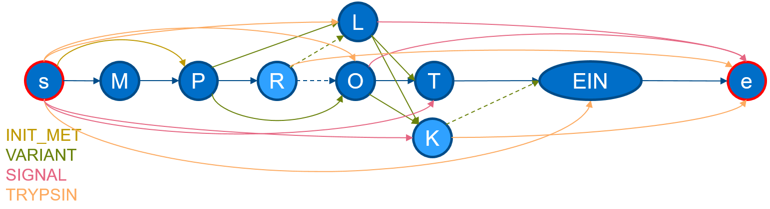The visualization shows, that the information from the section FT and SQ was added. The chain in the middle describes the canonical sequence. Additional nodes are added illustrating aminoacid-substitutions of the VARIANTs and additional edges have been added to mimic a SIGNAL-peptide. ProtGraph additionally adds a start node and a end node (internally denoted by: __start__ and __end__) and digested it by Trypsin (which is the default for each protein-graph).

All graphs generated by ProtGraph are so called directed and acyclic. These properties allow us to calculate interesting statistics about this protein:

E.G.: Executing protgraph -cnp examples/QXXXXX.txt adds the number of possible (non-repeating) paths between the start- and end-node into the statistics-output. We retrieve that there are 46 possible paths or in other words peptides in this graph.

E.G.: Executing protgraph -cnpm examples/QXXXXX.txt would include the number of possible paths binned by miscleavages into the statistics-output. This protein-graph contains 23 peptides with no miscleavages, 19 peptides with exactly 1 miscleavage and 4 peptides with exactly 2 miscleavages.

As seen in the image, ProtGraph, merges some nodes into a single node (e.g. EIN). We can prevent this behavior with the --no-merge-flag. Combining this flag with another, we can bin the number of paths by the path-length itself with protgraph -nm -cnph examples/QXXXXX.txt. The statistics-output would contain the total number of individual peptide-lengths within this protein-graph:

Peptide Length	1	2	3	4	5	6	7	8
#Peptides	3	5	8	8	6	4	8	4

Exporting Protein-Graphs to various graph-file-formats

While executing ProtGraph, generated graphs are not saved, which is the default behavior. We directly exclude the generated protein-graphs. To export each protein-graph into a file, simply set the flags -edot, -egraphml and/or -egml, which will create the corresponding dot, GraphML or GML files. Other tools, like Gephi, could then visualize this graph. With the flag -epickle it is also possible to generate a binary pickle file of a protein-graph (which can be used by other python programs). This is illustrated on the example protein QXXXXX:

$ protgraph -epickle examples/QXXXXX.txt 
1proteins [00:02,  2.05s/proteins]

To load the protein-graph back into python, it is enough to do the following:

In [1]: import pickle

In [2]: with open("exported_graphs/QXXXXX.pickle", "rb") as in_file:
   ...:     qxxxxx = pickle.load(in_file)

In [3]: qxxxxx
Out[3]: <igraph.Graph at 0x7f98b848e6b0>

In [4]: qxxxxx.vcount()
Out[4]: 10

In [5]: qxxxxx.ecount()
Out[5]: 24

In [6]: list(qxxxxx.vs[:])
Out[6]: 
[igraph.Vertex(<igraph.Graph object at 0x7f98b848e6b0>, 0, {'aminoacid': '__start__', 'position': 0, 'accession': 'QXXXXX'}),
 igraph.Vertex(<igraph.Graph object at 0x7f98b848e6b0>, 1, {'aminoacid': 'M', 'position': 1, 'accession': 'QXXXXX'}),
 igraph.Vertex(<igraph.Graph object at 0x7f98b848e6b0>, 2, {'aminoacid': 'P', 'position': 2, 'accession': 'QXXXXX'}),
 igraph.Vertex(<igraph.Graph object at 0x7f98b848e6b0>, 3, {'aminoacid': 'R', 'position': 3, 'accession': 'QXXXXX'}),
 igraph.Vertex(<igraph.Graph object at 0x7f98b848e6b0>, 4, {'aminoacid': 'O', 'position': 4, 'accession': 'QXXXXX'}),
 igraph.Vertex(<igraph.Graph object at 0x7f98b848e6b0>, 5, {'aminoacid': 'T', 'position': 5, 'accession': 'QXXXXX'}),
 igraph.Vertex(<igraph.Graph object at 0x7f98b848e6b0>, 6, {'aminoacid': '__end__', 'position': 9, 'accession': 'QXXXXX'}),
 igraph.Vertex(<igraph.Graph object at 0x7f98b848e6b0>, 7, {'aminoacid': 'L', 'position': None, 'accession': 'QXXXXX'}),
 igraph.Vertex(<igraph.Graph object at 0x7f98b848e6b0>, 8, {'aminoacid': 'K', 'position': None, 'accession': 'QXXXXX'}),
 igraph.Vertex(<igraph.Graph object at 0x7f98b848e6b0>, 9, {'aminoacid': 'EIN', 'position': 6, 'accession': 'QXXXXX'})]

Retrieving Statistics over the Tryptic Search Space of a Species (E.Coli)

In the example-folder you can find an already download SP-EMBL-entries of Escherichia coli (strain K12). Generating protein-graphs and a basic statistics-file over all entries can be calculated in seconds:

$ protgraph examples/e_coli.dat 
9434proteins [00:15, 627.51proteins/s] 

ProtGraph shows us that 9344 proteins have been processed. An excerpt of the basic statistics file informs us that ProtGraph included 28 isoforms, 815 signal peptides and 5034 mutagenic information. To include and retrieve the number of peptides for E.Coli we have to set the corresponding flags in ProtGraph and can then summarize the corresponding columns in the statistics file:

$ protgraph -nm -cnp -cnpm -cnph examples/e_coli.dat 
9434proteins [00:27, 348.70proteins/s]

$ protgraph_print_sums -cidx 12 protein_graph_statistics.csv 
9433rows [00:00, 135774.65rows/s]
Results from column 'num_paths':

Sum of each entry
0:  14842148316403611
....

$ protgraph_print_sums -cidx 13 protein_graph_statistics.csv 
9433rows [00:00, 19692.29rows/s]
Results from column 'list_paths_miscleavages':

Sum of each entry
  0:          24884044
  1:          80527605
  2:         126597315
  3:         152794276
...

$ protgraph_print_sums -cidx 14 protein_graph_statistics.csv 
9433rows [00:00, 19696.70rows/s]
Results from column 'list_paths_hops':

Sum of each entry
   0:                 0
   1:             32342
   2:             31252
   3:             31277
   4:             31303
   5:             30733
   6:             29118
   7:             30827
   8:             30653
   9:             30127
  10:             30780
...

From the output, it can be seen that already the proteins in E.Coli can yield 14842148316403611 peptides, if including all feature-information. The other outputs show, that we can bin those peptides by the number of miscleavages (e.g. exactly 24 884 044 peptides with 0 miscleavages) and by the peptide length (e.g. exactly 31 252 peptides with 2 aminoacids).

Replacing Aminoacids (J->I,L)

In some protein-entries provided by UniProtKB, some aminoacids are summarized by a single letter code. E.G.: the letter B corresponds to the aminoacid D (Aspartic acid) or N (Asparagine). ProtGraph can replace such aminoacids with the actual one as depicted below:

$ protgraph -cnp -raa "B->D,N" examples/e_coli.dat
9434proteins [00:16, 588.38proteins/s] 
$ protgraph_print_sums -cidx 12 protein_graph_statistics.csv 
9433rows [00:00, 142756.67rows/s]
Results from column 'num_paths':

Sum of each entry
0:  14842148316404547
...

$ protgraph -cnp -raa "J->I,L" examples/e_coli.dat
9434proteins [00:14, 671.71proteins/s] 
$ protgraph_print_sums -cidx 12 protein_graph_statistics.csv 
9433rows [00:00, 180680.48rows/s]
Results from column 'num_paths':

Sum of each entry
0:  14842148316403617
...

protgraph -cnp -raa "Z->Q,E" examples/e_coli.dat
9434proteins [00:06, 1560.85proteins/s]
$ protgraph_print_sums -cidx 12 protein_graph_statistics.csv 
9433rows [00:00, 197856.01rows/s]
Results from column 'num_paths':

Sum of each entry
0:  14842148316373256
...

$ protgraph -cnp -raa "X->A,C,D,E,F,G,H,I,K,L,M,N,O,P,Q,R,S,T,U,V,W,Y" examples/e_coli.dat
9434proteins [00:06, 1560.41proteins/s]
$ protgraph_print_sums -cidx 12 protein_graph_statistics.csv 
9433rows [00:00, 199515.24rows/s]
Results from column 'num_paths':

Sum of each entry
0:  14842148528266967
...

It can be observed that the number of peptides for E.Coli (tryptically digested) increases, since it now considers all possibilities of the substitutes in a sequence. The aminoacid-replacements (-raa) can also be chained and works for all aminoacids.

Generation of a E.Coli-FASTA-databases, containing only specific information

There are other formats like spectral libraries and alike but we first focused on the FASTA-format, since it is broadly used. ProtGraph traverses the proteins-graphs in a depth-search-manner and limits can be specified globally over a set of SP-EMBL-entries.

First, we generate a FASTA-file from the SP-EMBL-entries of E.Coli. It should only contain the canonical sequence (so no feature-information applied on the protein-graphs) and should be undigested:

$ protgraph -ft NONE -d skip -epepfasta --pep_fasta_out e_coli.fasta examples/e_coli.dat 
9434proteins [00:05, 1869.91proteins/s]

$ head e_coli.fasta 
>pg|ID_9|P13445(1:330,mssclvg:-1)
MSQNTLKVHDLNEDAEFDENGVEVFDEKALVEQEPSDNDLAEEELLSQGATQRVLDATQL
YLGEIGYSPLLTAEEEVYFARRALRGDVASRRRMIESNLRLVVKIARRYGNRGLALLDLI
EEGNLGLIRAVEKFDPERGFRFSTYATWWIRQTIERAIMNQTRTIRLPIHIVKELNVYLR
TARELSHKLDHEPSAEEIAEQLDKPVDDVSRMLRLNERITSVDTPLGGDSEKALLDILAD
EKENGPEDTTQDDDMKQSIVKWLFELNAKQREVLARRFGLLGYEAATLEDVGREIGLTRE
RVRQIQVEGLRRLREILQTQGLNIEALFRE
>pg|ID_3|P0A840(1:253,mssclvg:-1)
MRILLSNDDGVHAPGIQTLAKALREFADVQVVAPDRNRSGASNSLTLESSLRTFTFENGD
IAVQMGTPTDCVYLGVNALMRPRPDIVVSGINAGPNLGDDVIYSGTVAAAMEGRHLGFPA

$ cat e_coli.fasta | grep "^>" | wc -l
9434

NOTE: The generated FASTA-files using -epepfasta can have same sequences for multiple entries!

The FASTA-file contains the same number of entries as in the SP-EMBL-file. It can be noticed, that the header-format was reformatted to contain all the information along the path. pg stands for ProtGraph, the ID_XXX-describes an unique identifier for this FASTA-entry followed by the information along the path. In this case, it tells us the whole sequence of a Protein and that it had no miscleavages (which is true, since the protein-graph was not digested). Next, it would be interesting to export a digested FASTA-file (peptide-FASTA), containing SIGNAL-, PEPTIDE- and PROPEP-information:

$ protgraph -ft SIGNAL -ft PROPEP -ft PEPTIDE -d trypsin -epepfasta --pep_fasta_out e_coli_signal_propep_pep.fasta examples/e_coli.dat 
9434proteins [00:29, 324.64proteins/s]

$ head e_coli_signal_propep_pep.fasta 
>pg|ID_0|P23857(4:4,mssclvg:0)
K
>pg|ID_11|P23857(4:104,mssclvg:12)
KGLLALALVFSLPVFAAEHWIDVRVPEQYQQEHVQGAINIPLKEVKERIATAVPDKNDTV
KVYCNAGRQSGQAKEILSEMGYTHVENAGGLKDIAMPKVKG
>pg|ID_22|P23857(4:103,mssclvg:11)
KGLLALALVFSLPVFAAEHWIDVRVPEQYQQEHVQGAINIPLKEVKERIATAVPDKNDTV
KVYCNAGRQSGQAKEILSEMGYTHVENAGGLKDIAMPKVK
>pg|ID_33|P23857(4:101,mssclvg:10)
KGLLALALVFSLPVFAAEHWIDVRVPEQYQQEHVQGAINIPLKEVKERIATAVPDKNDTV

$ cat e_coli_signal_propep_pep.fasta | grep "SIGNAL" | head -n 1
>pg|ID_143|P23857(4:19,mssclvg:1,SIGNAL[1:19])

$ cat e_coli_signal_propep_pep.fasta | grep "^>" | wc -l
6660482

This FASTA-file is significantly larger (1.7 GB, containing ~6.6 million peptides) but contains all resulting peptides using the selected features while considering up to infinite many miscleavages. The output shows that the smallest peptides (like K) are also considered. Additionally, one entry is showcased resulting from a SIGNAL-peptide-feature. Since we considered a FASTA without any limitation, we now limit the minimum and maximum peptide length to 6-60 and allow up to 2 miscleavages:

$ protgraph -nm -ft SIGNAL -ft PROPEP -ft PEPTIDE -d trypsin --pep_miscleavages 2 --pep_min_pep_length 6 --pep_hops 60 -epepfasta --pep_fasta_out e_coli_with_selected_features_limited.fasta examples/e_coli.dat 
9434proteins [00:14, 671.77proteins/s] 

$ head e_coli_with_selected_features_limited.fasta
>pg|ID_8|P0A840(1:24,mssclvg:2)
MRILLSNDDGVHAPGIQTLAKALR
>pg|ID_19|P0A840(1:21,mssclvg:1)
MRILLSNDDGVHAPGIQTLAK
>pg|ID_30|P0A840(22:38,mssclvg:2)
ALREFADVQVVAPDRNR
>pg|ID_41|P0A840(22:36,mssclvg:1)
ALREFADVQVVAPDR
>pg|ID_52|P0A840(130:151,mssclvg:2)
HYDTAAAVTCSILRALCKEPLR

$ cat e_coli_with_selected_features_limited.fasta| grep "^>" | wc -l
648551

We can see that the number peptides within this FASTA is significantly reduced (to ~650 000 entries). NOTE: for setting an upper length-limit of peptides we need to set -nm. In case of not setting this parameter, longer peptides may be exported. Finally, since the FASTA-file still contains for some entries same sequences, we can concatenate these by using a different (and more sophisticated) FASTA-exporter:

$ protgraph -nm -ft SIGNAL -ft PROPEP -ft PEPTIDE -d trypsin --pep_miscleavages 2 --pep_min_pep_length 6 --pep_hops 60 -epepsqlite --pep_sqlite_database e_coli_database.db examples/e_coli.dat 
9434proteins [00:16, 587.41proteins/s] 

$ protgraph_pepsqlite_to_fasta -o e_coli_compact.fasta e_coli_database.db 
100%|███████████████| 404212/404212 [00:00<00:00, 511718.70entries/s]

$ head e_coli_compact.fasta
>pg|ID_0|P0A840(1:24,mssclvg:2),A0A4S5AWU9(1:24,mssclvg:2)
MRILLSNDDGVHAPGIQTLAKALR
>pg|ID_1|P0A840(1:21,mssclvg:1),A0A4S5AWU9(1:21,mssclvg:1)
MRILLSNDDGVHAPGIQTLAK
>pg|ID_2|P0A840(22:38,mssclvg:2),A0A4S5AWU9(22:38,mssclvg:2)
ALREFADVQVVAPDRNR
>pg|ID_3|P0A840(22:36,mssclvg:1),A0A4S5AWU9(22:36,mssclvg:1)
ALREFADVQVVAPDR
>pg|ID_4|P0A840(130:151,mssclvg:2),A0A4S5AWU9(130:151,mssclvg:2)
HYDTAAAVTCSILRALCKEPLR

$ cat e_coli_compact.fasta | grep "^>" | wc -l
404212

Instead of directly generating a FASTA-file we first create a database, summarizing same sequences and headers. As a post-processing step, the database-entries are exported into FASTA. The generated FASTA has unique sequence as entries and offers some additionally insights. From the first entries we see peptides shared by exactly 2 proteins. Looking at the difference between the compact and non-compact FASTA, we see that ~244 000 entries could be summarized into already included entries in the FASTA. This generated FASTA-file can be used for identification.

NOTE: Protein-Graphs can contain large amounts of peptides/proteins. Do a dry run with the flags -cnp, -cnpm or cnph (or all of them) WITHOUT the export functionality first and examine the statistics output if it is feasible to generate a FASTA-file. Without a dry run it may happen that a protein like P04637 (P53 Human) with all possible peptides and variants is exported, which will very likely take up all your disk space.