Multiple instruments
One of the most requested features to be included in kima is the possibility to analyse RV data from multiple instruments. This is now possible!
Notes
-
This feature is available in the master branch as of kima v2.0.
Still, some bugs 🐛 may be left to catch. Let us know if you find one. -
Considering RVs from multiple instruments means adding new offset parameters
to the model. As of now, all these parameters share the same prior. -
The same applies to the additional white noise (sometimes called jitter ).
One jitter parameter is added per instrument, all sharing the same prior.
First announced by Fischer et al. 2002, the giant planet orbiting HD106252 has been detected with a number of different instruments (Perrier et al. 2003, Butler et al. 2006, Wittenmyer et al.2009). In this small tutorial, we will analyse the combined RV data.
If you have a recent version of kima (after v2.0, commit e599ffd), there's no setting up required.
The old instructions to checkout the multi_instrument branch were moved to the end of this page.
Head over to the examples/multi_instrument directory.
There you will find four files containing the RV data of HD106252,
each of them from a different instrument:
HD106252_ELODIE.txt, HD106252_HET.txt, HD106252_HJS.txt, and HD106252_Lick.txt.
You will note that each file has a different number of observations,
but the header occupies the same two lines in each.
When reading the data into kima, it is important to guarantee
that the structure, header, and units of all the data files are the same.
For each file, the first column is time in (Julian) days, second column is RV in m/s, and third column is RV uncertainty also in m/s.
In that directory there is another file called HD106252_joined.txt,
which contains the same RV data of the four instruments, but joined together.
The structure of the three first columns is identical, but the fourth column
contains an instrument (integer) identifier.
kima is able to read these two types of input: one file per instrument, or one single file with an identifier (integer!) column.
The kima_setup.cpp file contains mostly the usual code to define a model.
One difference is the new option
const bool multi_instrument = true; which tells kima that the RVs come from different instruments.
As mentioned above, this means defining new offset parameters. The default (shared) prior for these parameters is a uniform distribution within the span of the observed RVs (see here)
This is usually a good option which guarantees that the prior contains the full range of possible values for the offsets, whether they are positive or negative. But bear in mind that you might have to adjust this prior for your data.
The next new thing is when reading the data. To read the four individual files we can do
datafiles = {"HD106252_ELODIE.txt",
             "HD106252_HET.txt",
             "HD106252_HJS.txt",
             "HD106252_Lick.txt"
            };

load_multi(datafiles, "ms", 2);
In case we want to read the file with the joined RVs, we could use instead
datafile = "HD106252_joined.txt";
load_multi(datafile, "ms", 1);[note: the load_multi function is overloaded to deal with
char* and vector<char*>. The other two arguments are the same.]
[note: the data should be read in only one of these ways, not both!]
Now that we're all set, let's compile and run the model
make # may be compiled already
./run
With the default options, the sampler will finish in about 15 minutes, give or take. Remember that you can check the progress and look at the results while the code is running, by opening a new terminal window. Do give it some time at the start, as this example takes a bit to "converge".
Let's use pykima to look at the results. The command
kima-showresults all
will create a number of different plots. Some interesting ones are reproduced here:
- the posterior for the orbital period, showing a very clear peak close to 1535 days.

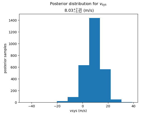
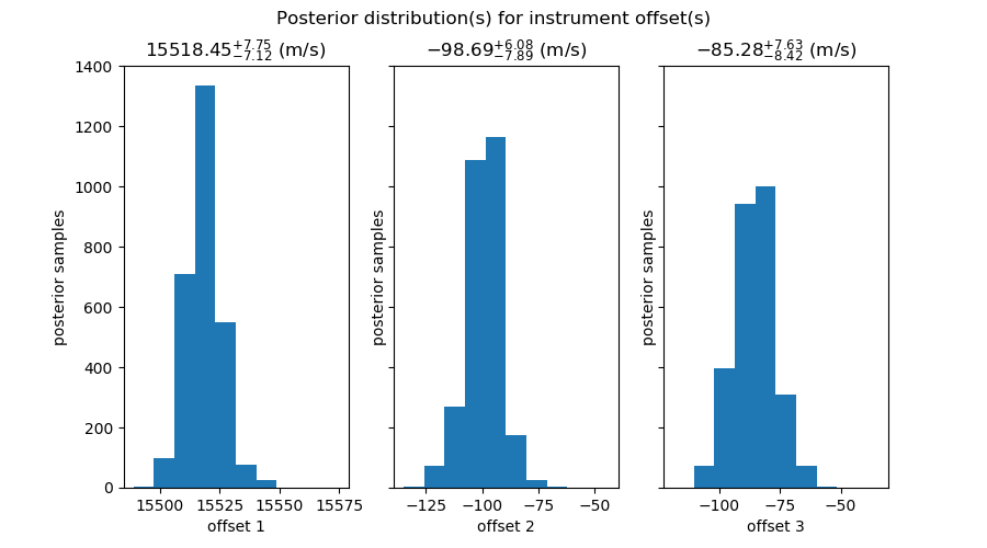
- the posteriors for the systemic velocity and the (3) between-instrument offsets
- the posterior for the jitter parameters

- the phased RV curve, based on the maximum likelihood solution
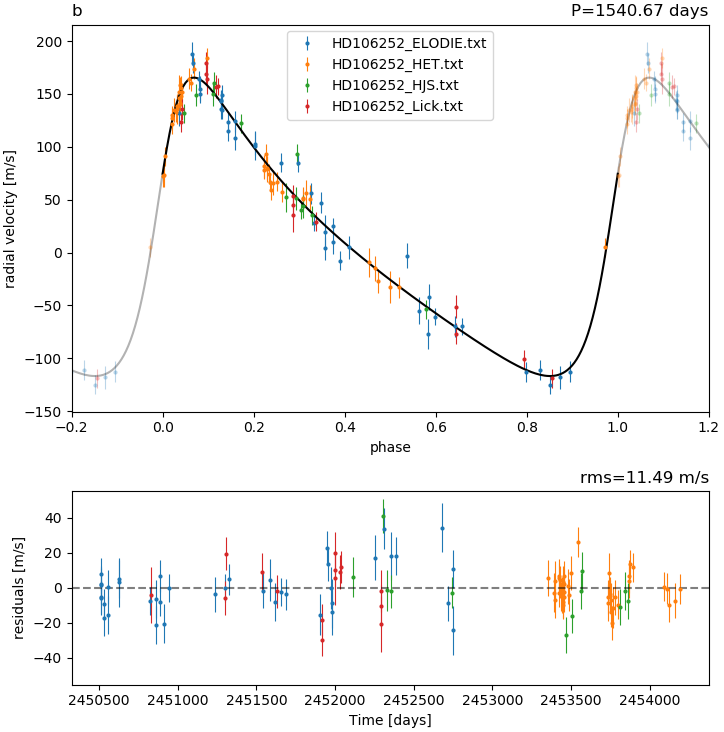
- and finally the RV curves together with the data from each instrument
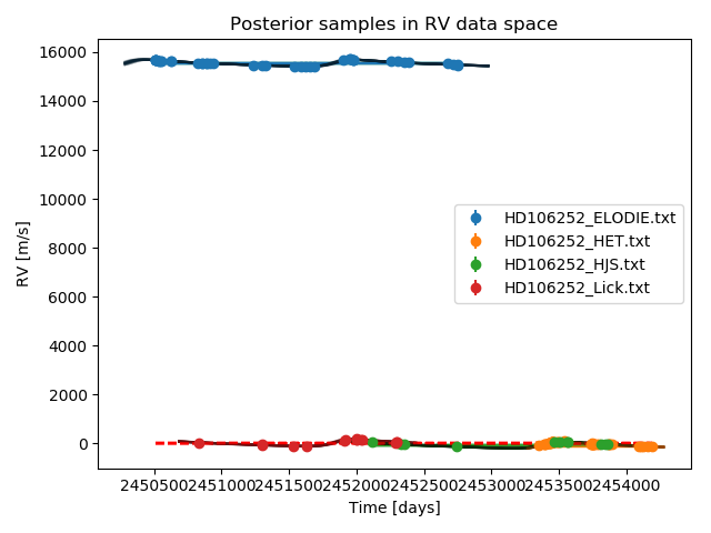
Zooming in on this last plot, we see how each dataset is modelled with the same Keplerian function plus an individual offset
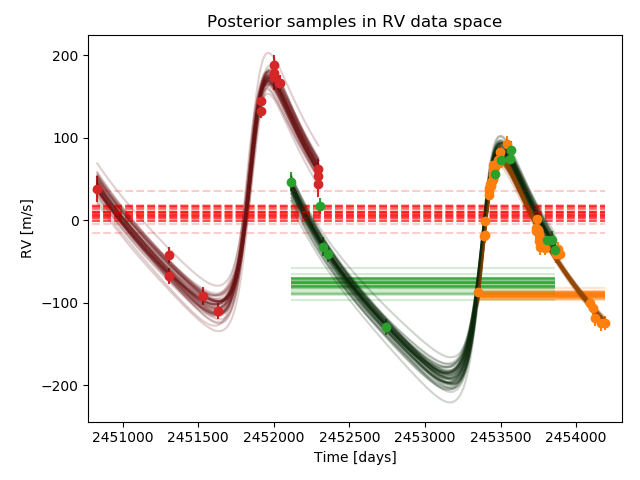
To clarify, in the multi_instrument mode, with Ni instruments, there are
- Ni-1 offset parameters
- Ni jitter parameters
- 1 systemic velocity
The correspondence between these parameters
can be worked out by looking at the order of the files in the datafiles vector.
The systemic velocity is associated with the last instrument
(Lick in the above example, shown in red in the plot).
The RV offsets are then defined relative to the systemic velocity.
So, offset1 is between Lick and ELODIE data (blue),
offset2 is between Lick and HET data (orange),
and offset3 is between LICK and HJS data (green).
The jitter parameters are simply in the same order as the
instruments in the datafiles vector: ELODIE, HET, HJS, and Lick.