cynet

Info

See <https://arxiv.org/abs/1406.6651> for theoretical background

Author

ZeD@UChicago <zed.uchicago.edu>

Description

Implementation of the Deep Granger net inference algorithm, described in https://arxiv.org/abs/1406.6651, for learning spatio-temporal stochastic processes (point processes). cynet learns a network of generative local models, without assuming any specific model structure.

Note

If issues arise with dependencies in python3, be sure that tkinter is installed

sudo apt-get install python3-tk

Usage:

from cynet import cynet
from cynet.cynet import uNetworkModels as models
from viscynet import viscynet as vcn

cynet module includes:

• cynet
• viscynet

cynet library classes:

• spatioTemporal
• uNetworkModels
• simulateModels
• xgModels

Examples of Pipeline:

You may find two examples of this pipeline in your enviroment's bin folder after installing the cynet package. There will also be a pdf walking through another extremely detailed example.

Produces detailed timeseries predictions using Deep Granger Nets.

Description of Pipeline:

You may find two examples of this pipeline in your enviroment's bin folder after installing the cynet package.

Step 1:

Use the spatioTemporal class and its utility functions to fit and manipulate your data into a timeseries grid. The end outputs will be triplets: files that contain the rows (coordinates), the columns (dates), and the timeseries. The splitTS function will help generate rows of the timeseries. Generally, we use this to create timeseries beyond the length of the data in the triplets. We use the triplets to generate predictive models and then split, which have the longer timeseries to evaluate those models.

Step 2:

Run xGenESeSS on the triplets to generate predictive models. The xgModels class can be used to assist in this step. If running on a cluster, set run local to false and calling xgModels.run() will generate the shell commands to run xGenESeSS in a text file. Otherwise, xgModels will run locally using the binary installed with the package. The end result are predictive models. Note that example 1 starts at this point. Thus there are sample models provided.

Step 3:

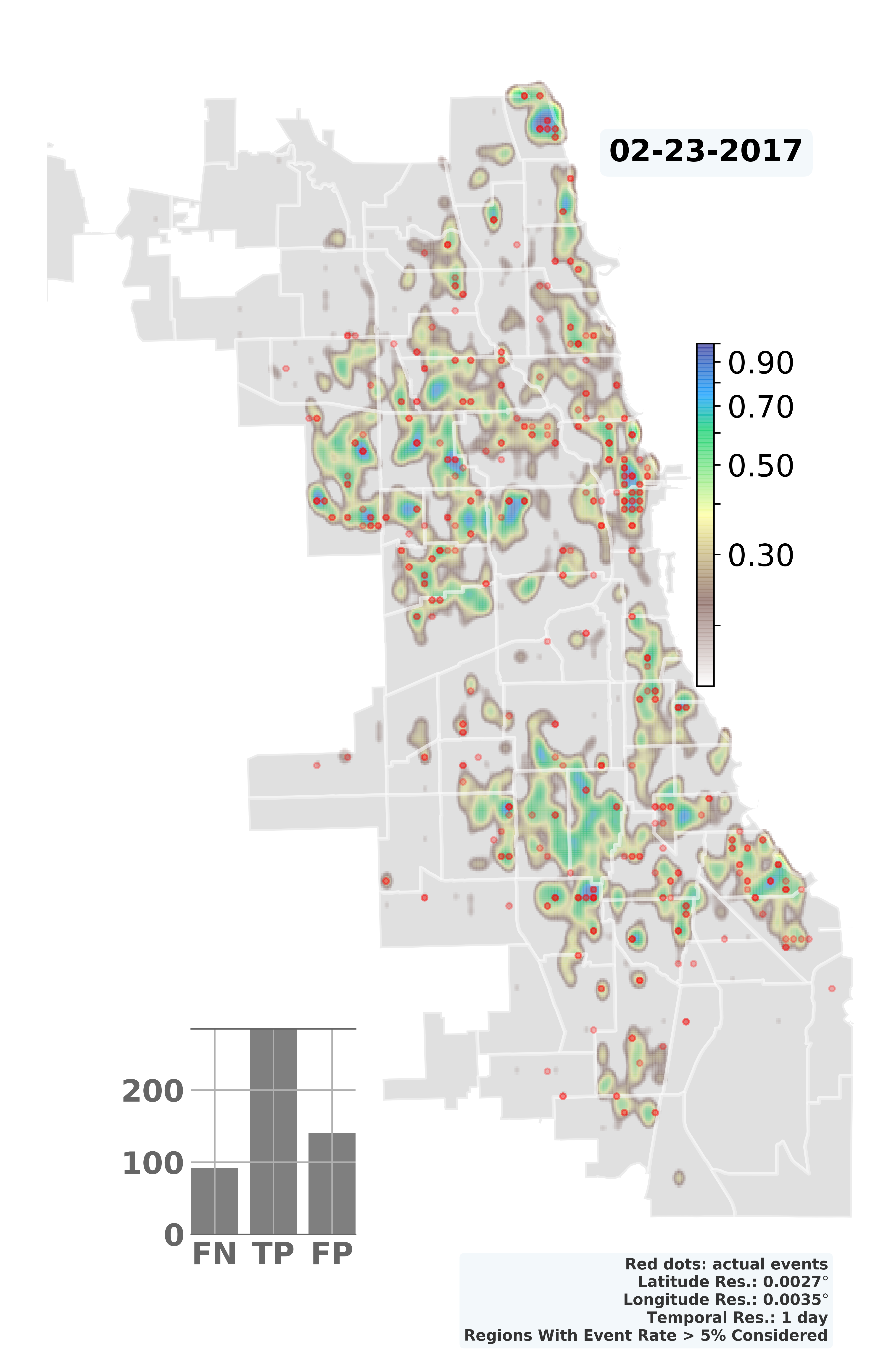
To evaluate the models afterwards, use the run_pipeline utility function. This calls uNetworkModels and simulateModels in parallel to evaluate each model. simulateModels calls the cynet and flexroc binaries. Outputs will be auc, tpr, and fpr statistics.

See example 2 for an example of the entire pipeline.