NB: Original README can be found below
News: I have merged the PR from @AU-Nebula that (hopefully) make it easier to set up and run. Thank @AU-Nebula!
The current KERN implementation relies on CUDA 9.0 which, unfortunately, is an older version that does not run on more recent operating systems. Regardless of your operating system's support for CUDA 9.0, begin with the following steps:
- Clone the repository:
git clone https://github.com/yuweihao/KERN.git. - Change directory:
cd KERN. - Run:
sh kern_setup.sh. There are quite some data to download, so this step will take a while. The script assumes that Docker and NVIDIA Container Toolkit are installed on the system. - Activate the Conda environment:
conda activate kern. - Compile the CUDA part of the project:
sh compile.sh. - Generate knowledge matrices (statistical prior):
python prior_matrices/generate_knowledge.py. - Test KERN processing by running Validation task with VG dataset:
python models/eval_rels.py -ckpt checkpoints/kern_sgdet.tar.
- Run:
docker run -it -v $PWD:/kern --gpus all cuda9. - Upload custom dataset to
/data/custom_images. - Run:
sh scripts/eval_kern_sgdet.sh.
- Create visualization script for Custom Dataset
the Setup section in the original README below.
Tianshui Chen*, Weihao Yu*, Riquan Chen, and Liang Lin, “Knowledge-Embedded Routing Network for Scene Graph Generation”, CVPR, 2019. (* co-first authors) [PDF]
Note A typo in our final CVPR version paper: h_{iC}^o in eq. (6) should be corrected to f_{iC}^o.
This repository contains trained models and PyTorch version code for the above paper, If the paper significantly inspires you, we request that you cite our work:
@inproceedings{chen2019knowledge,
  title={Knowledge-Embedded Routing Network for Scene Graph Generation},
  author={Chen, Tianshui and Yu, Weihao and Chen, Riquan and Lin, Liang},
  booktitle = "Conference on Computer Vision and Pattern Recognition",
  year={2019}
}
In our paper, our model's strong baseline model is SMN (Stacked Motif Networks) introduced by @rowanz et al. To compare these two models fairly, the PyTorch version code of our model is based on @rowanz's code neural-motifs. Thank @rowanz for sharing his nice code to research community.
-
Install python3.6 and pytorch 3. I recommend the Anaconda distribution. To install PyTorch if you haven't already, use
conda install pytorch=0.3.0 torchvision=0.2.0 cuda90 -c pytorch. We use TensorBoard to observe the results of validation dataset. If you want to use it in PyTorch, you should install TensorFlow and tensorboardX first. If you don't want to use TensorBaord, just not use the command-tb_log_dir. -
Update the config file with the dataset paths. Specifically:
- Visual Genome (the VG_100K folder, image_data.json, VG-SGG.h5, and VG-SGG-dicts.json). See data/stanford_filtered/README.md for the steps to download these.
- You'll also need to fix your PYTHONPATH:
export PYTHONPATH=/home/yuweihao/exp/KERN
-
Compile everything. Update your CUDA path in Makefile file and run
makein the main directory: this compiles the Bilinear Interpolation operation for the RoIs. -
Pretrain VG detection. To compare our model with neural-motifs fairly, we just use their pretrained VG detection. You can download their pretrained detector checkpoint provided by @rowanz. You could also run ./scripts/pretrain_detector.sh to train detector by yourself. Note: You might have to modify the learning rate and batch size according to number and memory of GPU you have.
-
Generate knowledge matrices:
python prior_matrices/generate_knowledge.py, or download them from here: prior_matrices (Google Drive, OneDrive). -
Train our KERN model. There are three training phase. You need a GPU with 12G memory.
- Train VG relationship predicate classification: run
CUDA_VISIBLE_DEVICES=YOUR_GPU_NUM ./scripts/train_kern_predcls.shThis phase maybe last about 20-30 epochs. - Train scene graph classification: run
CUDA_VISIBLE_DEVICES=YOUR_GPU_NUM ./scripts/train_kern_sgcls.sh. Before run this script, you need to modify the path name of best checkpoint you trained in precls phase:-ckpt checkpoints/kern_predcls/vgrel-YOUR_BEST_EPOCH_RNUM.tar. It lasts about 8-13 epochs, then you can decrease the learning rate to 1e-6 to further improve the performance. Like neural-motifs, we use only one trained checkpoint for both predcls and sgcls tasks. You can also download our checkpoint here: kern_sgcls_predcls.tar (Google Drive, OneDrive). - Refine for detection: run
CUDA_VISIBLE_DEVICES=YOUR_GPU_NUM ./scripts/train_kern_sgdet.shor download the checkpoint here: kern_sgdet.tar (Google Drive, OneDrive). If you find the validation performance plateaus, you could also decrease learning rate to 1e-6 to improve performance.
- Train VG relationship predicate classification: run
-
Evaluate: refer to the scripts
CUDA_VISIBLE_DEVICES=YOUR_GPU_NUM ./scripts/eval_kern_[predcls/sgcls/sgdet].sh. You can conveniently find all our checkpoints, evaluation caches and results in this folder KERN_Download (Google Drive, OneDrive).
In validation/test dataset, assume there are images. For each image, a model generates top
predicted relationship triplets. As for image
, there are
ground truth relationship triplets, where
triplets are predicted successfully by the model. We can calculate:
For image , in its
ground truth relationship triplets, there are
ground truth triplets with relationship
(Except
, meaning no relationship. The number of relationship classes is
, including no relationship), where
triplets are predicted successfully by the model. In
images of validation/test dataset, for relationship
, there are
images which contain at least one ground truth triplet with this relationship. The R@X of relationship
can be calculated:
Then we can calculate:
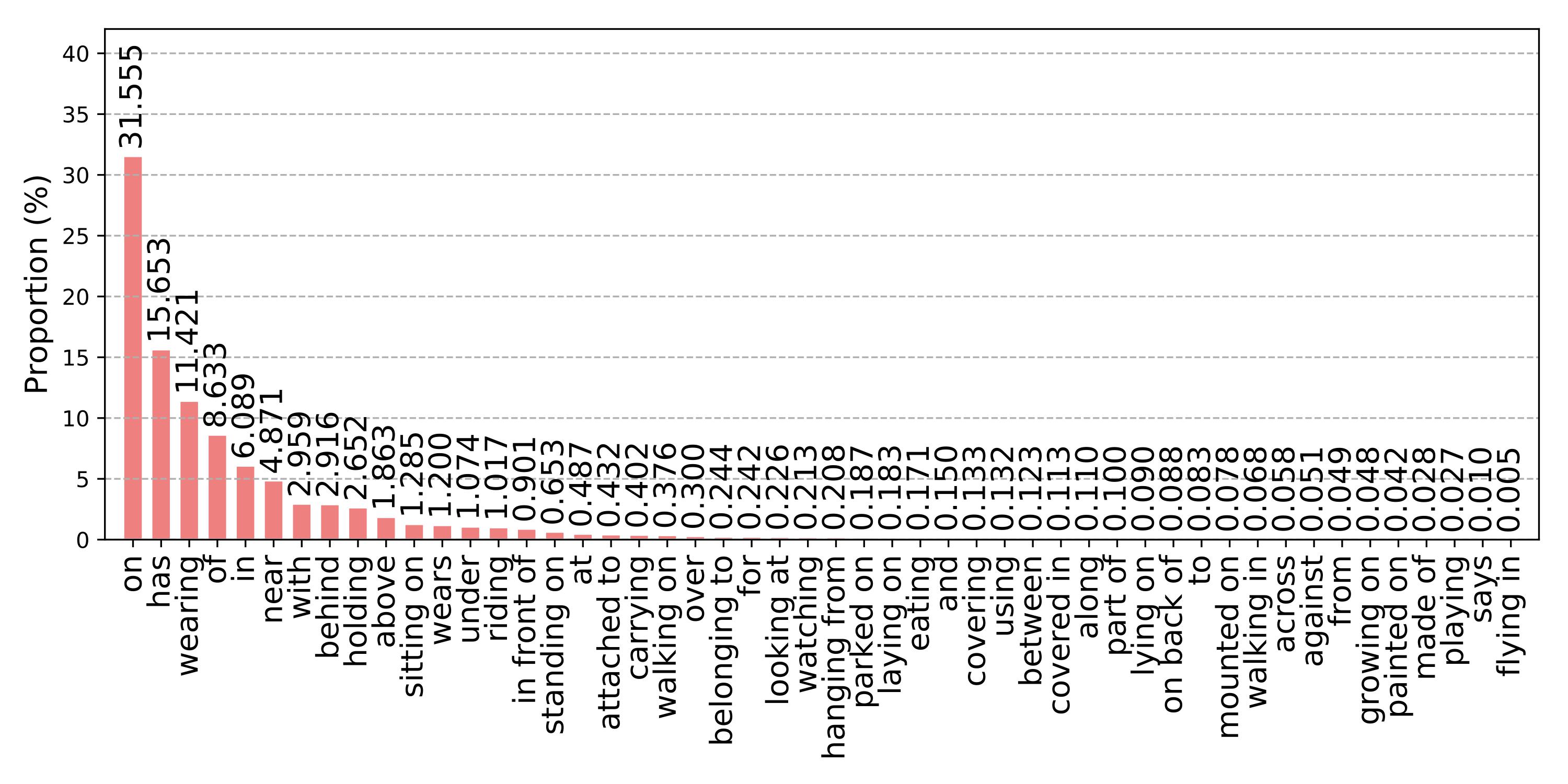 Figure 1. The distribution of different relationships on the VG dataset. The training and test splits share similar distribution.
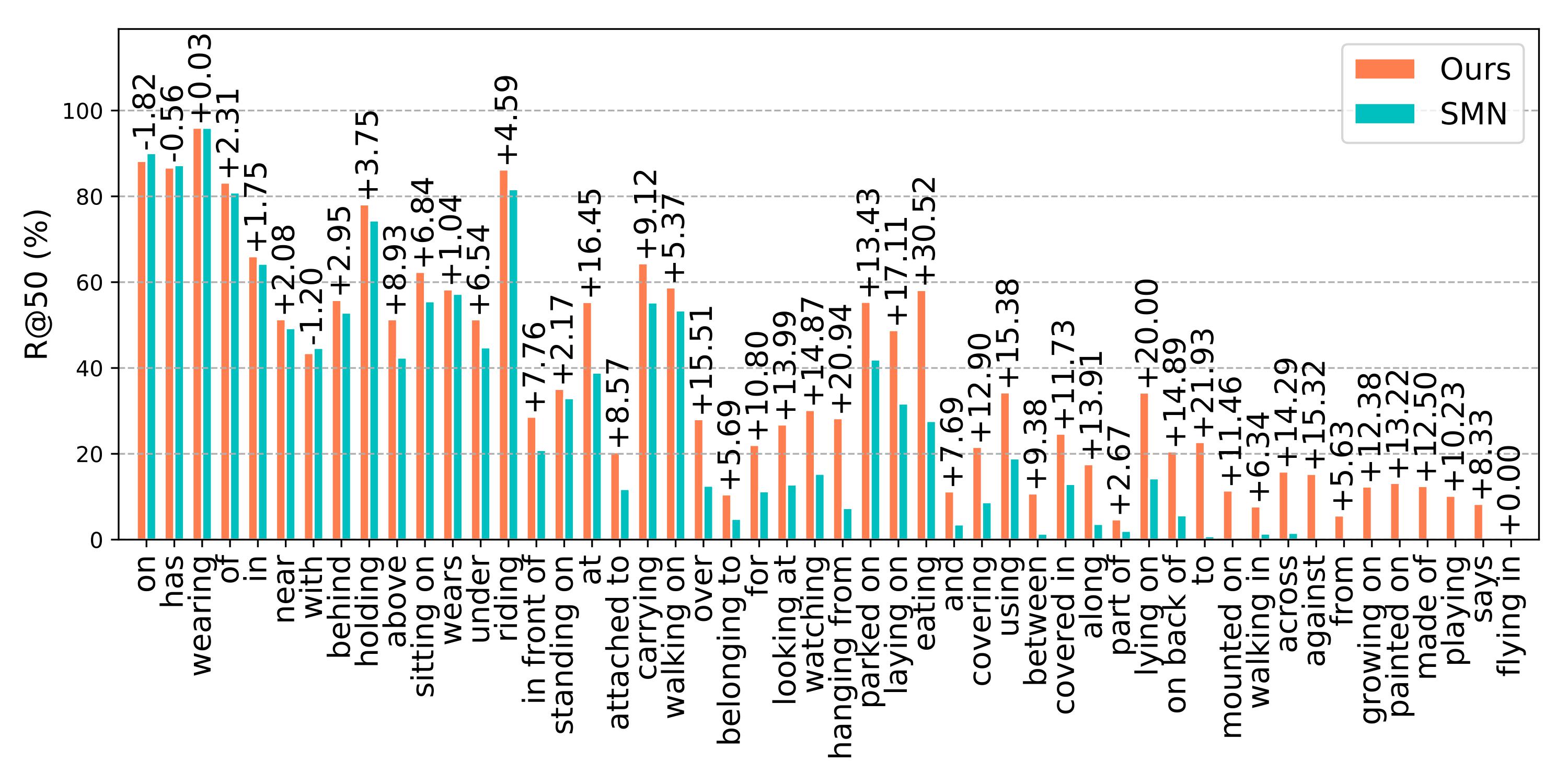 Figure 2. The R@50 without constraint of our method and the SMN on the predicate classification task on the VG dataset.
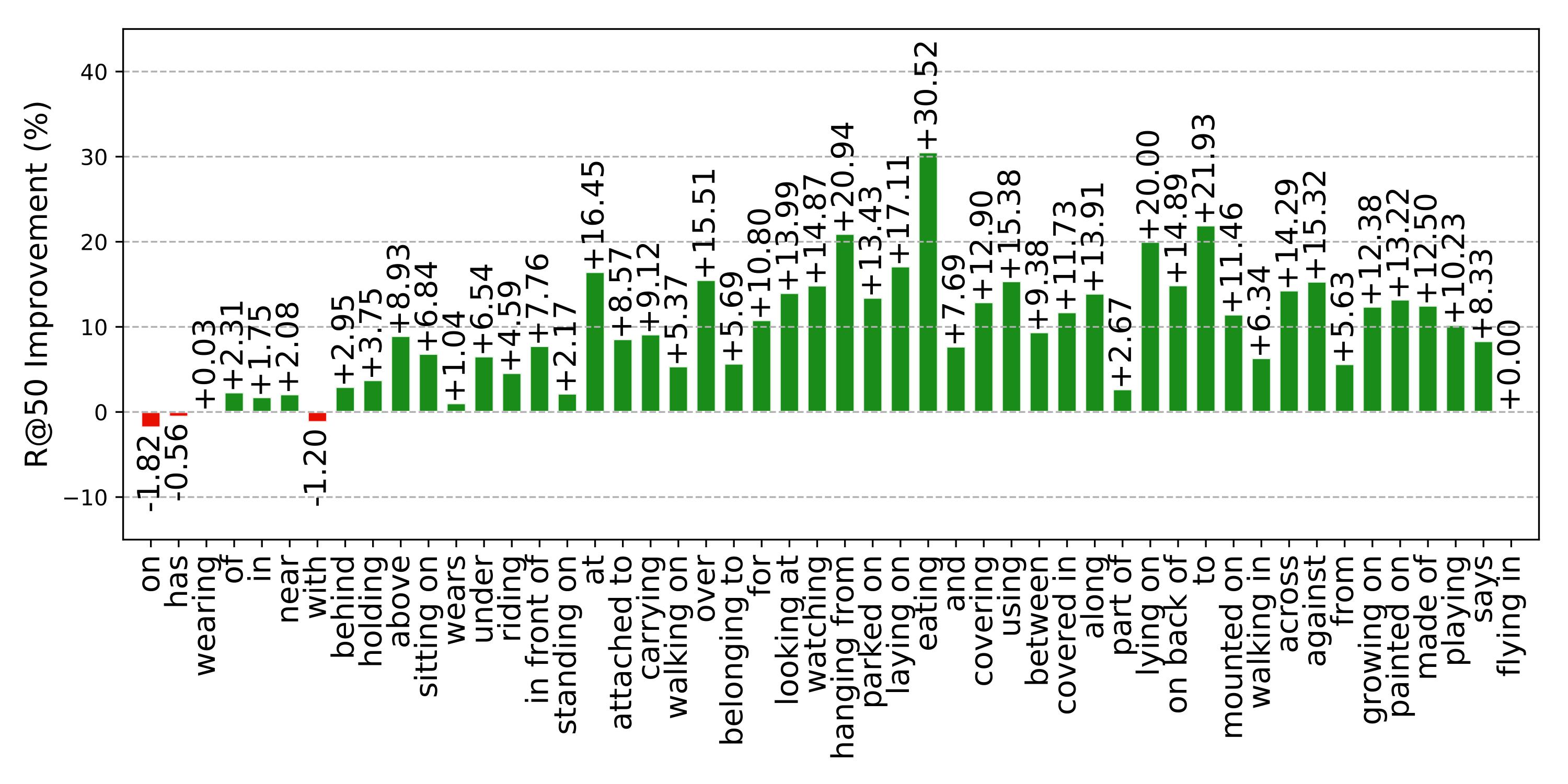 Figure 3. The R@50 absolute improvement of different relationships of our method to the SMN. The R@50 are computed without constraint.
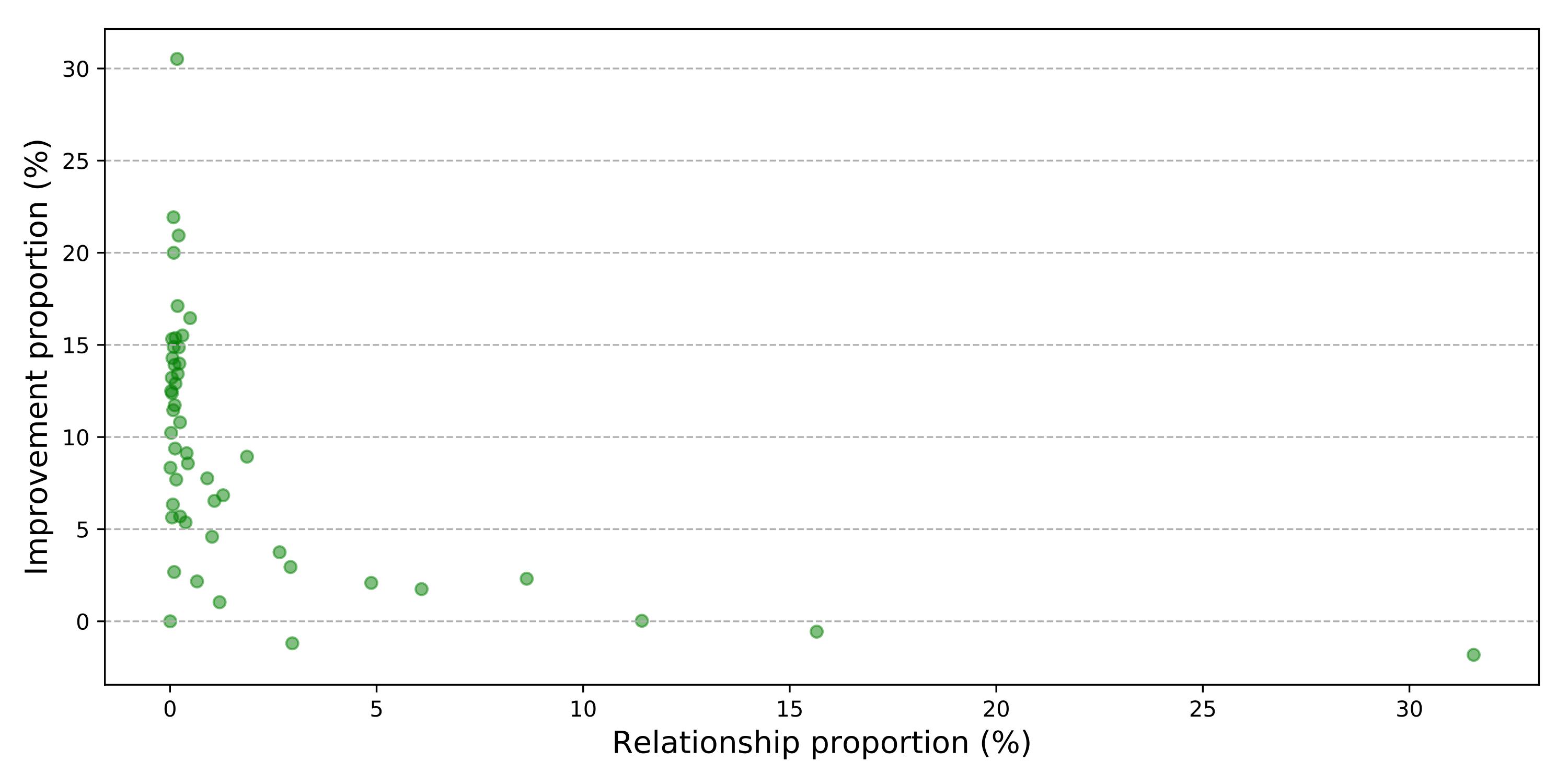 Figure 4. The relation between the R@50 improvement and sample proportion on the predicate classification task on the VG dataset. The R@50 are computed without constraint.
| Method | SGGen | SGCls | PredCls | Mean | Relative | ||||
| mR@50 | mR@100 | mR@50 | mR@100 | mR@50 | mR@100 | improvement | |||
| Constraint | SMN | 5.3 | 6.1 | 7.1 | 7.6 | 13.3 | 14.4 | 9.0 | |
| Ours | 6.4 | 7.3 | 9.4 | 10.0 | 17.7 | 19.2 | 11.7 | ↑ 30.0% | |
| Unconstraint | SMN | 9.3 | 12.9 | 15.4 | 20.6 | 27.5 | 37.9 | 20.6 | |
| Ours | 11.7 | 16.0 | 19.8 | 26.2 | 36.3 | 49.0 | 26.5 | ↑ 28.6% |
Thank @rowanz for his generously releasing nice code neural-motifs.
Feel free to open an issue if you encounter trouble getting it to work.