SymJava is a Java library for symbolic-numeric computation.
There are two unique features which make SymJava different:
-
Operator Overloading is implemented by using Java-OO (https://github.com/amelentev/java-oo)
-
Java bytecode is generated at runtime for symbolic expressions which make the numerical evaluation really fast.
Install java-oo Eclipse plugin for Java Operator Overloading support (https://github.com/amelentev/java-oo): Click in menu: Help -> Install New Software. Enter in "Work with" field: http://amelentev.github.io/eclipse.jdt-oo-site/
If you are using Eclipse-Kepler you need to install SR2 4.3.2 here https://www.eclipse.org/downloads/packages/release/kepler/sr2)
If you are using Eclipse 4.4+, you need Scalar IDE plugin. see https://github.com/amelentev/java-oo
Both Java 7 and 8 are supported.
If you were using Futureye_JIT for academic research, you are encouraged to cite the following papers:
package symjava.examples;

import static symjava.symbolic.Symbol.*;
import symjava.bytecode.BytecodeFunc;
import symjava.symbolic.*;

/**
 * This example uses Java Operator Overloading for symbolic computation.
 * See https://github.com/amelentev/java-oo for Java Operator Overloading.
 *
 */
public class Example1 {

	public static void main(String[] args) {
		Expr expr = x + y * z;
		System.out.println(expr); //x + y*z

		Expr expr2 = expr.subs(x, y*y);
		System.out.println(expr2); //y^2 + y*z
		System.out.println(expr2.diff(y)); //2*y + z

		Func f = new Func("f1", expr2.diff(y));
		System.out.println(f); //2*y + z

		BytecodeFunc func = f.toBytecodeFunc();
		System.out.println(func.apply(1,2)); //4.0
	}
}
package symjava.examples;
import symjava.relational.Eq;
import symjava.symbolic.Symbol;
import static symjava.symbolic.Symbol.*;
public class Example2 {
/**
* Example from Wikipedia
* (http://en.wikipedia.org/wiki/Gauss-Newton_algorithm)
*
* Use Gauss-Newton algorithm to fit a given model y=a*x/(b-x)
*
*/
public static void example1() {
//Model y=a*x/(b-x), Unknown parameters: a, b
Symbol[] freeVars = {x};
Symbol[] params = {a, b};
Eq eq = new Eq(y, a*x/(b+x), freeVars, params);
//Data for (x,y)
double[][] data = {
{0.038,0.050},
{0.194,0.127},
{0.425,0.094},
{0.626,0.2122},
{1.253,0.2729},
{2.500,0.2665},
{3.740,0.3317}
};
double[] initialGuess = {0.9, 0.2};
//Here we go ...
GaussNewton.solve(eq, initialGuess, data, 100, 1e-4);
}
/**
* Example from Apache Commons Math
* (http://commons.apache.org/proper/commons-math/userguide/optimization.html)
*
* "We are looking to find the best parameters [a, b, c] for the quadratic function
*
* f(x) = a x2 + b x + c.
*
* The data set below was generated using [a = 8, b = 10, c = 16]. A random number
* between zero and one was added to each y value calculated. "
*
*/
public static void example2() {
Symbol[] freeVars = {x};
Symbol[] params = {a, b, c};
Eq eq = new Eq(y, a*x*x + b*x + c, freeVars, params);
double[][] data = {
{1 , 34.234064369},
{2 , 68.2681162306108},
{3 , 118.615899084602},
{4 , 184.138197238557},
{5 , 266.599877916276},
{6 , 364.147735251579},
{7 , 478.019226091914},
{8 , 608.140949270688},
{9 , 754.598868667148},
{10, 916.128818085883},
};
double[] initialGuess = {1, 1, 1};
GaussNewton.solve(eq, initialGuess, data, 100, 1e-4);
}
public static void main(String[] args) {
example1();
example2();
}
}Output in Latex:
Jacobian Matrix =

Residuals =

Iterativly sovle ...
a=0.33266 b=0.26017
a=0.34281 b=0.42608
a=0.35778 b=0.52951
a=0.36141 b=0.55366
a=0.36180 b=0.55607
a=0.36183 b=0.55625
Jacobian Matrix =

Residuals =

Iterativly sovle ...
a=7.99883 b=10.00184 c=16.32401
package symjava.examples;

import Jama.Matrix;
import symjava.matrix.*;
import symjava.relational.Eq;
import symjava.symbolic.Expr;

/**
 * A general Gauss Newton solver using SymJava for simbolic computations
 * instead of writing your own Jacobian matrix and Residuals
 */
public class GaussNewton {

	public static void solve(Eq eq, double[] init, double[][] data, int maxIter, double eps) {
		int n = data.length;

		//Construct Jacobian Matrix and Residuals
		SymVector res = new SymVector(n);
		SymMatrix J = new SymMatrix(n, eq.getParams().length);

		Expr[] params = eq.getParams();
		for(int i=0; i<n; i++) {
			Eq subEq = eq.subsUnknowns(data[i]);
			res[i] = subEq.lhs - subEq.rhs; //res[i] =y[i] - a*x[i]/(b + x[i]);
			for(int j=0; j<eq.getParams().length; j++) {
				Expr df = res[i].diff(params[j]);
				J[i][j] = df;
			}
		}

		System.out.println("Jacobian Matrix = ");
		System.out.println(J);
		System.out.println("Residuals = ");
		System.out.println(res);

		//Convert symbolic staff to Bytecode staff to speedup evaluation
		NumVector Nres = new NumVector(res, eq.getParams());
		NumMatrix NJ = new NumMatrix(J, eq.getParams());

		System.out.println("Iterativly sovle ... ");
		for(int i=0; i<maxIter; i++) {
			//Use JAMA to solve the system
			Matrix A = new Matrix(NJ.eval(init));
			Matrix b = new Matrix(Nres.eval(init), Nres.dim());
			Matrix x = A.solve(b); //Lease Square solution
			if(x.norm2() < eps)
				break;
			//Update initial guess
			for(int j=0; j<init.length; j++) {
				init[j] = init[j] - x.get(j, 0);
				System.out.print(String.format("%s=%.5f",eq.getParams()[j], init[j])+" ");
			}
			System.out.println();
		}
	}
}
package symjava.examples;
import static symjava.symbolic.Symbol.*;
import symjava.relational.Eq;
import symjava.symbolic.*;
public class Example3 {
/**
* Square root of a number
* (http://en.wikipedia.org/wiki/Newton's_method)
*/
public static void example1() {
Expr[] freeVars = {x};
double num = 612;
Eq[] eq = new Eq[] {
new Eq(x*x-num, C0, freeVars, null)
};
double[] guess = new double[]{ 10 };
Newton.solve(eq, guess, 100, 1e-3);
}
/**
* Example from Wikipedia
* (http://en.wikipedia.org/wiki/Gauss-Newton_algorithm)
*
* Use Lagrange Multipliers and Newton method to fit a given model y=a*x/(b-x)
*
*/
public static void example2() {
//Model y=a*x/(b-x), Unknown parameters: a, b
Symbol[] freeVars = {x};
Symbol[] params = {a, b};
Eq eq = new Eq(y - a*x/(b+x), C0, freeVars, params);
//Data for (x,y)
double[][] data = {
{0.038,0.050},
{0.194,0.127},
{0.425,0.094},
{0.626,0.2122},
{1.253,0.2729},
{2.500,0.2665},
{3.740,0.3317}
};
double[] initialGuess = {0.9, 0.2};
LagrangeMultipliers lm = new LagrangeMultipliers(eq, initialGuess, data);
//Just for purpose of displaying summation expression
Eq L = lm.getEqForDisplay();
System.out.println("L("+SymPrinting.join(L.getUnknowns(),",")+")=\n "+L.lhs);
System.out.println("where data array is (X_i, Y_i), i=0..."+(data.length-1));
NewtonOptimization.solve(L, lm.getInitialGuess(), 100, 1e-4, true);
Eq L2 = lm.getEq();
System.out.println("L("+SymPrinting.join(L.getUnknowns(),",")+")=\n "+L2.lhs);
NewtonOptimization.solve(L2, lm.getInitialGuess(), 100, 1e-4, false);
}
public static void main(String[] args) {
example1();
example2();
}
}Jacobian Matrix =
\left[ {\begin{array}{c}
2*x\\
\end{array} } \right]
Iterativly sovle ...
x=10.00000
x=35.60000
x=26.39551
x=24.79064
x=24.73869
Output in Latex:
Lagrange=

where data array is (X_i, Y_i), i=0...6
Hessian=

Grad(L)=

Iterativly sovle ...
y_0=0.00000 y_1=0.00000 y_2=0.00000 y_3=0.00000 y_4=0.00000 y_5=0.00000 y_6=0.00000 \lambda_0=0.00000 \lambda_1=0.00000 \lambda_2=0.00000 \lambda_3=0.00000 \lambda_4=0.00000 \lambda_5=0.00000 \lambda_6=0.00000 a=0.90000 b=0.20000
y_0=0.01678 y_1=0.09612 y_2=0.16729 y_3=0.20243 y_4=0.25473 y_5=0.28945 y_6=0.30273 \lambda_0=0.06643 \lambda_1=0.06176 \lambda_2=-0.14658 \lambda_3=0.01955 \lambda_4=0.03634 \lambda_5=-0.04590 \lambda_6=0.05794 a=0.33266 b=0.26017
y_0=0.01624 y_1=0.08735 y_2=0.15765 y_3=0.19518 y_4=0.25469 y_5=0.29667 y_6=0.31327 \lambda_0=0.06752 \lambda_1=0.07930 \lambda_2=-0.12729 \lambda_3=0.03404 \lambda_4=0.03642 \lambda_5=-0.06034 \lambda_6=0.03687 a=0.35178 b=0.46125
y_0=0.02256 y_1=0.09240 y_2=0.15593 y_3=0.19116 y_4=0.25076 y_5=0.29644 y_6=0.31550 \lambda_0=0.05487 \lambda_1=0.06919 \lambda_2=-0.12387 \lambda_3=0.04207 \lambda_4=0.04428 \lambda_5=-0.05989 \lambda_6=0.03240 a=0.36223 b=0.55462
y_0=0.02314 y_1=0.09356 y_2=0.15671 y_3=0.19159 y_4=0.25059 y_5=0.29598 y_6=0.31499 \lambda_0=0.05373 \lambda_1=0.06689 \lambda_2=-0.12542 \lambda_3=0.04123 \lambda_4=0.04463 \lambda_5=-0.05896 \lambda_6=0.03342 a=0.36185 b=0.55631
package symjava.examples;
 import static symjava.symbolic.Symbol.*;
import symjava.matrix.*;
import symjava.symbolic.*;
 /**
 * Example for PDE Constrained Parameters Optimization
 *
 */
public class Example4 {
	public static void main(String[] args) {
		Func u =  new Func("u",  x,y,z);
		Func u0 = new Func("u0", x,y,z);
		Func q =  new Func("q",  x,y,z);
		Func q0 = new Func("q0", x,y,z);
		Func f =  new Func("f",  x,y,z);
		Func lamd = new Func("\\lambda ", x,y,z);

		Expr reg_term = (q-q0)*(q-q0)*0.5*0.1;
 		Func L = new Func("L",(u-u0)*(u-u0)/2 + reg_term + q*Dot.apply(Grad.apply(u), Grad.apply(lamd)) - f*lamd);
		System.out.println("Lagrange L(u, \\lambda, q) = \n"+L);

		Func phi = new Func("\\phi ", x,y,z);
		Func psi = new Func("\\psi ", x,y,z);
		Func chi = new Func("\\chi ", x,y,z);
		Expr[] xs =  new Expr[]{u,   lamd, q   };
		Expr[] dxs = new Expr[]{phi, psi,  chi };
		SymVector Lx = Grad.apply(L, xs, dxs);
		System.out.println("\nGradient Lx = (Lu, Llamd, Lq) =");
		System.out.println(Lx);

		Func du = new Func("\\delta{u}", x,y,z);
		Func dl = new Func("\\delta{\\lambda}", x,y,z);
		Func dq = new Func("\\delta{q}", x,y,z);
		Expr[] dxs2 = new Expr[] { du, dl, dq };
		SymMatrix Lxx = new SymMatrix();
		for(Expr Lxi : Lx) {
			Lxx.add(Grad.apply(Lxi, xs, dxs2));
		}
		System.out.println("\nHessian Matrix =");
		System.out.println(Lxx);
	}
}
Output in Latex:
Lagrange=
 Hessian=
 Grad(L)=

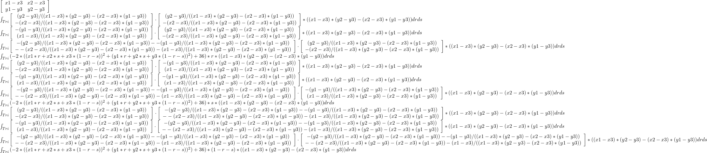
Example6: Finite Element Solver for Laplace Equation