Breast Cancer Detection using Machine Learning

Sajjad Salaria

Feb 8 · 5 min read

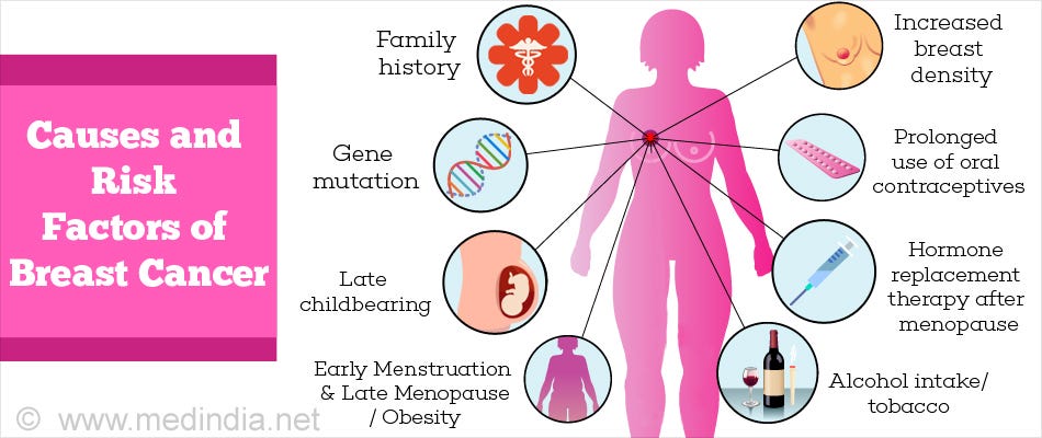
Breast cancer the most common cancer among women worldwide accounting for 25 percent of all cancer cases and affected 2.1 million people in 2015 early diagnosis significantly increases the chances of survival.
The key challenge in cancer detection is how to classify tumors into malignant or benign machine learning techniques can dramatically improves the accuracy of diagnosis

Research indicates that most experienced physicians can diagnose cancer with 79 percent accuracy while 91 percent correct diagnosis is achieved using machine learning techniques.

word cloud

In this case study, our task is to classify tumors into malignant or benign tumors using features of pain from several cell images.

Let’s take a look at the cancer diagnosis and classification process.
So the first step in the cancer diagnosis process is to do what we call it final needle aspirate or if any process which is simply extracting some of the cells out of the tumor. And at that stage, we don’t know if that human is malignant or benign. When you say malignant or benign as you guys can see these are kind of the images of the this would be benign tumor and this is the malignant tumor. And when we say benign that means that the tumor is kind of not spreading across the bodies of the patient is safe somehow.
It’s if it’s malignant That means it’s it’s a cancerous.

That means we need to intervene and actually stop the cancer growth
And what we do here in the machine learning aspect so now as we extracted all these images and we wanted to specify if that cancer out of these images is malignant or benign that’s the whole idea.
So what we do with that we extract out of these images some features when we see features that mean some characteristics out of the image such as radius, for example the cells such as texture perimeter area smoothness and so on. And then we feed all these features into kind of our machine learning model in a way which is kind of a brain in a way.

The idea is to teach the machine how to basically classify images or classify data and tell us OK if it’s malignant or benign for example in this case without any human intervention which is going to change the model once the model is trained we’re good to go we can use it in practice to classify new images as we move forward. And that’s kind of the overall procedure or the cancer diagnosis procedure.

STEP #1: PROBLEM STATEMENT

• Predicting if the cancer diagnosis is benign or malignant based on several observations/features
• 30 features are used, examples:
• - radius (mean of distances from center to points on the perimeter)
• - texture (standard deviation of gray-scale values) - perimeter
• - area - smoothness (local variation in radius lengths)
• - compactness (perimeter^2 / area - 1.0)
• - concavity (severity of concave portions of the contour)
• - concave points (number of concave portions of the contour)
• - symmetry
• - fractal dimension ("coastline approximation" - 1)
• Datasets are linearly separable using all 30 input features
• Number of Instances: 569
• Class Distribution: 212 Malignant, 357 Benign
• Target class:
• - Malignant - Benign

STEP #2: IMPORTING DATA

import libraries

import pandas as pd # Import Pandas for data manipulation using dataframes
import numpy as np # Import Numpy for data statistical analysis
import matplotlib.pyplot as plt # Import matplotlib for data visualisation
import seaborn as sns # Statistical data visualization

%matplotlib inline

Import dataset

Import Cancer data drom the Sklearn library

from sklearn.datasets import load_breast_cancer
cancer = load_breast_cancer()

STEP #3: VISUALIZING THE DATA

sns.pairplot(df_cancer, hue = 'target', vars = ['mean radius', 'mean texture', 'mean area', 'mean perimeter', 'mean smoothness'] )

sns.countplot(df_cancer['target'], label = "Count")

HeatMap

Let's check the correlation between the variables

Strong correlation between the mean radius and mean perimeter, mean area and mean primeter

plt.figure(figsize=(20,10))
sns.heatmap(df_cancer.corr(), annot=True)

Heatmap of datset

STEP #4: MODEL TRAINING

Let's drop the target label coloumns

X = df_cancer.drop(['target'],axis=1)from sklearn.model_selection import train_test_splitX_train, X_test, y_train, y_test = train_test_split(X, y, test_size = 0.20, random_state=5)

STEP #5: EVALUATING THE MODEL

y_predict = svc_model.predict(X_test)
cm = confusion_matrix(y_test, y_predict)sns.heatmap(cm, annot=True)

print(classification_report(y_test, y_predict))

---

STEP #6: IMPROVING THE MODEL

min_train = X_train.min()range_train = (X_train - min_train).max()X_train_scaled = (X_train - min_train)/range_trainsns.scatterplot(x = X_train['mean area'], y = X_train['mean smoothness'], hue = y_train)from sklearn.svm import SVC
from sklearn.metrics import classification_report, confusion_matrixsvc_model = SVC()
svc_model.fit(X_train_scaled, y_train)y_predict = svc_model.predict(X_test_scaled)
cm = confusion_matrix(y_test, y_predict)sns.heatmap(cm,annot=True,fmt="d")

print(classification_report(y_test,y_predict))

---

images: https://goo.gl/m812UK, www.medindia.net