Modelling Early User-Game Interactions for Joint Estimation of Survival Time and Churn Probability

Repository hosting a minimal version of the code employed for the paper:

Modelling Early User-Game Interactions for Joint Estimation of Survival Time and Churn Probability

Overview

The aim of this work was to develop a more generalizable and holistic methodlogy for modelling user engagement which at the same time possessed characteristics appealing for industry applications. In this view we tried to achieve a series of applicative goals:

APPLICATIVE GOALS

Create a methodology:

1 Able to jointly estimate engagement related behaviours (i.e. churn probability and survival time) given a restricted number of observations and features.
2 Able to scale well when considering large volumes of data.
3 Having noise-resilience properties.
4 Easy to integrate in larger frameworks.
5 Able to express uncertainty around its estimates.

Other than trying to accomplish the aformetioned technical objectives, the present project attempted to test a series of theoretical assumptions:

THEORETICAL GOALS

1 Non-linear models are more suitable than linear for estimating behaviours arising from complex processes like engagement.
2 Churn probability and survival time can be modelled as arising from a common underlying process (i.e. the engagement process).
3 The aforementioned process can be expressed through a minimal set of features representing frequency and ammount of behavioural activity.
4 Explicitly modelling the temporal dynamics in the aformentioned behavioural features allows to better estimate churn probability and survival time, supposedly due to a better approximation of the underlying engagement process.

Proposed Model

Here a graphical reppresentation of the Deep Neural Network architecture we designed and developed for achieving the aformetioned goals

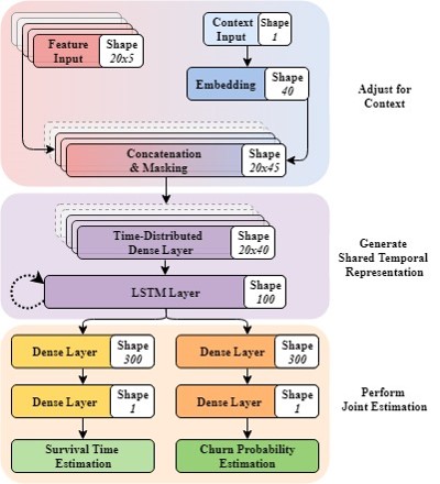
The first section aims to learn an embedding for each game context and fusing it with a restricted number of features indicative of behavioural activity. This is achieved concatenating the two tensors and applying a set of non-linear transformations in a time-distributed way.

The context embedding allows the model to learn a rich multi-dimensional representation of each considered game projecting similar games into closer points in the latent space. This allows to appropriately weight the behavioural features according to the context to which they belong. In this way, the model has the ability to become more proficient and more genralizable the more contexts are provided at training time.

The second section takes this fused representation over time and models it temporally using a Recurrent Neural Network (RNN) employing Long Short-Term Memory (LSTM) cells. The use of a RNN is particularly suitable here because it can handle time series of different lengths and explicitly model temporal dependencies between the inputs.

We thought to use this part of the model for extracting a high level representation of the player state which could be used for predicting measures of future disengagement and sustained engagement. This was achieved by ’branching’ two shallow Neural Networks tasked to perform churn probability and survival time estimation.

Data

Due to commerical sensitivity and data protection regulations we are not allowed to pubblicly release the data employed in the present work.

However, due to the principles that guided our features selection process (i.e. generalizability and proximity to behavioural primitives), we believe that our methodology can be easily tested on a wide range of data sources with minimal or no adjustments.

For running minimal_test.py the follwoing structure in the data folder should be respected:

n=Number of data points
k=Total number of unique contexts taken into consideration
t=Maximum number of time-steps taken into consideration

data   
│
└───collapsed
|
│   X_tr.npy        |   shape=(n, 5+k)  |   Training set features + one-hot encode of context
│   X_ts.npy        |   shape=(n, 5+k)  |   Test set features + one-hot encode of context
│   y_r_tr.npy      |   shape=(n, 1)    |   Training set regression target
│   y_r_ts.npy      |   shape=(n, 1)    |   Test set regression target
│   y_c_tr.npy      |   shape=(n, 1)    |   Training set classification target
│   y_c_ts.npy      |   shape=(n, 1)    |   Test set classification target
|   context_tr.npy  |   shape=(n, 1)    |   Training set context names
|   context_ts.npy  |   shape=(n, 1)    |   Test set context names
|
└───unfolded
|
│   X_tr.npy        |   shape=(n, (5*t)+k)  |   Training set features + one-hot encode of context
│   X_ts.npy        |   shape=(n, (5*t)+k)  |   Test set features + one-hot encode of context
│   y_r_tr.npy      |   shape=(n, 1)        |   Training set regression target
│   y_r_ts.npy      |   shape=(n, 1)        |   Test set regression target
│   y_c_tr.npy      |   shape=(n, 1)        |   Training set classification target
│   y_c_ts.npy      |   shape=(n, 1)        |   Test set classification target
|   context_tr.npy  |   shape=(n, 1)        |   Training set context names
|   context_ts.npy  |   shape=(n, 1)        |   Test set context names
|
└───temporal  
|
│   X_feat_tr.npy   |   shape=(n, t, 5)   |   Training set features (temporal format)
│   X_feat_ts.npy   |   shape=(n, t, 5)   |   Test set features (temporal format)
│   X_cont_tr.npy   |   shape=(n, 1)      |   Training set context features (numerical encoding)
│   X_cont_ts.npy   |   shape=(n, 1)      |   Test set context features (numerical encoding)
│   y_r_tr.npy      |   shape=(n, 1)      |   Training set regression target
│   y_r_ts.npy      |   shape=(n, 1)      |   Test set regression target
│   y_c_tr.npy      |   shape=(n, 1)      |   Training set classification target
│   y_c_ts.npy      |   shape=(n, 1)      |   Test set classification target
|   context_tr.npy  |   shape=(n, 1)      |   Training set context names
|   context_ts.npy  |   shape=(n, 1)      |   Test set context names

Results

PERFORMANCE

For the sake of brevity here we will report, for each estimator, only aggregated metrics over the 6 considered games. More detailed results can be found in the paper.

Churn Estimation

Estimator	Metric	Score	Score	Number of Parameters	Fitting Time (seconds)
		Mean	Std
bifurcating_temporal	f1	0.679	0.024	26902	2134.809
mlp_c_collapsed	f1	0.619	0.042	19081	108.205
logistic_collapsed	f1	0.613	0.033	17	22.767
logistic_unrolled	f1	0.611	0.031	107	25.281
mlp_c_unrolled	f1	0.604	0.098	27181	108.348
mean_model	f1	0.334	0.002	1	0

Survival Estimation

Estimator	Metric	Score	Score	Number of Parameters	Fitting Time (seconds)
		Mean	Std
bifurcating_temporal	smape	0.267	0.058	26902	2134.809
mlp_r_collapsed	smape	0.356	0.089	19081	109.536
mlp_r_unrolled	smape	0.357	0.096	27181	77.468
mean_model	smape	0.498	0.195	1	0
enet_collapsed	smape	0.519	0.205	17	169.825
enet_unrolled	smape	0.519	0.205	107	212.023

INSPECTING THE LEARNED USER EMBEDDING

One of the advantege of modelling engagement related behaviours as arising from a common underlying process is that we can interpret this last one as a reppresentation of the user state.

Usage

Using a model from models.py

Each model inherits from a protected AbstractEstimator class implementing methods which are shared among the various models (e.g. fit(), predict() ecc...). When instatiated each model needs to receive the feature (X) and target (y) arrays for inferring the input and output shapes of the underlying TensorFlow graph. For generating the TensorFlow graph (through Keras functional API) the generate_model() method needs to be called passing two dictionary: one describing the hyper-parameters (i.e. hp_schema) and another specifying the parameters for compiling the graph.

import numpy as np
from modules.models import MultilayerPerceptron as MLP

# random data
X = np.random.random(size=(10000, 100))
y = np.random.random(size=(10000, 1))

# define the model schemas
perceptron_c_schemas = {
  'hp_schema': {
    'layers': [90, 90, 90],
    'activation': 'relu',
    'dropout': 0.0
   },
  'comp_schema': {
    'optimizer': 'adam',
    'loss': 'binary_crossentropy',
    'metrics': ['acc']
   }
}

# instantiale the model class
perceptron_c = MLP(
  X_train=X,
  y_train=y
)

# generate the TensorFlow graph
perceptron_c.generate_model(
  hp_schema=perceptron_c_schemas['hp_schema'],
  comp_schema=perceptron_c_schemas['comp_schema'],
  regression=False,
  model_tag='my_perceptron_classifier'
)

# fit here is just a wrapper function for Keras fit() method
perceptron_c.fit(
  x=X,
  y=y,
  batch_size=256,
  epochs=10,
  validation_split=0.2
)

Running minimal_test.py

This is a script for fitting and comparing the various models presented in the paper, it will generate and save (in the results folder) a CSV file containing a more detailed version of table present in the Perfromance section.
The only requirements for running minimal_test.py are: having all the necessary libraries and having the relevant numpy arrays in the data folder.

Bare in mind that for running the script without any further change, minimal_test.py requires already pre-processed data in the previously defined shape.

Requirements

Either install the requirements on your local machine through pip install -r requirements.txt or create a virtual environment with:

# Pipenv is a virtual environment manager
pip install pipenv

# Create a virtual environment in this directory
pipenv install

# Open / activate virtual environment
pipenv shell

# Install all the dependencies
pip install -r requirements.txt
# Now we are good to go....

For Windows users we strongly advise to install numpy==1.17.1+mkl and scipy==1.3.1 (in this order) directly from the binaries distributed through https://www.lfd.uci.edu/~gohlke/pythonlibs.

Cite & Contact

Please cite this work as:

Bonometti, Valerio, Ringer, Charles, Hall, Mark, Wade, Alex R., Drachen, Anders (2019) Modelling Early User-Game Interactions for Joint Estimation of Survival Time and Churn Probability, In: Proceedings of the IEEE Conference on Games 2019. IEEE

Bibtex entry:

@inproceedings{bonometti2019modelling,
  title={Modelling early user-game interactions for joint estimation of survival time and churn probability},
  author={Bonometti, Valerio and Ringer, Charles and Hall, Mark and Wade, Alex R and Drachen, Anders},
  booktitle={2019 IEEE Conference on Games (CoG)},
  pages={1--8},
  year={2019},
  organization={IEEE}
}

Or get in touch with us at vb690@york.ac.uk, we are looking for collaboration opportunities.