amoeba2

Automated Molecular Excitation Bayesian line-fitting Algorithm

amoeba2 is based on AMOEBA and Petzler et al. (2021).

Given a set of optical depth spectra associated with the 1612, 1665, 1667, and 1720 MHz transitions of OH, amoeba2 uses a Monte Carlo Markov Chain analysis to infer the optimal number of Gaussian components and their parameters. Here is a basic outline of the algorithm:

0. First, amoeba2 calculates the Bayesian Information Criterion (BIC) over the data for the null hypothesis.

1. Starting with one component, amoeba2 will sample the posterior distribution using MCMC with at least 4 independent chains.

2. Because of the degeneracies related to fitting Gaussians (even constrained Gaussians!) to data, it is possible that chains get stuck in a local maximum of the posterior distribution. This is especially likely when the number of components is less than the "true" number of components, in which case each chain may decide to fit a different subset of the components. amoeba2 checks if the chains appear converged by evaluating the BIC over the data using the mean point estimate per chain. Any deviant chains are discarded.

3. There also exists a labeling degeneracy: each chain could decide to fit the components in a different order. To break the degeneracy, amoeba2 uses a Gaussian Mixture Model (GMM) to cluster the posterior samples of all chains into the same number of groups as there are expected components. It also tests fewer and more clusters and evaluates the BIC for each number of clusters in order to determine how many clusters appears optimal to explain the posterior samples.

4. Once completed, amoeba2 checks to see if the chains appear converged (by comparing the BIC of each chain's mean point estimate to that of the combined posterior samples) and if the number of components seems converged (by comparing the ideal GMM cluster count to the model number of components). If both convergence checks are passed, then amoeba2 will stop.

5. amoeba2 also checks to see if there were any divergences in the posterior sampling. Divergences in amoeba2 indicate that the model number of components exceeds the true number of components present in the data. If there are divergences, then amoeba2 will stop.

6. If the BIC of the mean point estimate has decreased compared to the previous iteration, then amoeba2 will fit another model with a different number of model components. The strategy is either to increment the number of components by one (see fit_all() below) or to try the number of components predicted by the GMM (see fit_best() below).

7. If the BIC of the mean point estimate increases two iterations in a row, then amoeba2 will stop.

Installation

conda create --name amoeba2 -c conda-forge pymc
conda activate amoeba2
pip install git+https://github.com/tvwenger/amoeba2.git

Usage

In general, try help(function) for a thorough explanation of the parameters, return values, and other information related to function (e.g., help(simulate_tau_spectra).

Synthetic Observations

The program simulate.py can be used to generate simulated data for testing.

import numpy as np
from amoeba2.simulate import simulate_tau_spectra

# Define velocity axes for each transition.
# In general, the order of things is 1612, 1665, 1667, and 1720 MHz
velocity_axes = [
    np.arange(-15.0, 15.1, 0.15), # 1612 MHz
    np.arange(-12.0, 12.1, 0.12), # 1665 MHz
    np.arange(-12.0, 12.1, 0.12), # 1667 MHz
    np.arange(-10.0, 10.1, 0.10), # 1720 MHz
]

# Define the "truths" for four spectral line components
truths = {
    "center": np.array([-1.5, -0.75, 0.15, 0.55]), # centroids
    "log10_fwhm": np.array(
        [np.log10(0.75), np.log10(1.0), np.log10(0.5), np.log10(0.75)]
    ), # log10 full-width at half-maximum line widths
    "peak_tau_1612": np.array([0.005, 0.025, -0.03, 0.015]), # peak optical depths
    "peak_tau_1665": np.array([0.02, -0.01, -0.002, 0.0]),
    "peak_tau_1667": np.array([-0.01, 0.015, -0.025, -0.025]),
}

# Set the optical depth rms in each transition
tau_rms = np.array([0.001, 0.0012, 0.0014, 0.0016])

# Evaluate simulated optical depth spectra
tau_spectra, truths = simulate_tau_spectra(
    velocity_axes,
    tau_rms,
    truths,
    seed=5391,
)
# truths now contains peak_tau_1720, which has been set by the
# optical depth sum rule.

Initializing the data structure

The data (either real or simulated) must be contained within a special amoeba2 data structure

from amoeba2.data import AmoebaData

# Initialize the data structure
data = AmoebaData()

# Add the data to the structure
for i, transition in enumerate(["1612", "1665", "1667", "1720"]):
    data.set_spectrum(
        transition,
        velocity_axes[i],
        tau_spectra[i],
        tau_rms[i],
    )

Single model demonstration

If the number of spectral components is known a priori, then a model may be fit.

from amoeba2.model import AmoebaTauModel

# Initialize the model
model = AmoebaTauModel(
    n_gauss=4, # number of components
    seed=1234, # random number generator seed
    verbose=True
)

# Set the prior distributions
# Normal distribution with mean = 0 and sigma = 1.0
model.set_prior("center", "normal", np.array([0.0, 1.0]))

# Normal distribution with mean = 0 and sigma = 0.25
model.set_prior("log10_fwhm", "normal", np.array([0.0, 0.25]))

# Normal distribution with mean = 0 and sigma = 0.25
model.set_prior("peak_tau", "normal", np.array([0.0, 0.01]))

# Add a Normal likelihood distribution
model.add_likelihood("normal")

# Add the data
model.set_data(data)
# N.B. you can update the data using this function instead of re-specifying
# the entire model (e.g., if your priors aren't changing between successive
# runs of amoeba2)

# Generate prior predictive samples to test the prior distribution validity
prior_predictive = model.prior_predictive_check(
    samples=50, plot_fname="prior_predictive.png"
)

# Sample the posterior distribution with 8 chains and 8 CPUs
# using 1000 tuning iterations and then drawing 1000 samples
model.fit(tune=1000, draws=1000, chains=8, cores=8)

# Plot the posterior sample chains
model.plot_traces("traces.png")

# Generate posterior predictive samples to check posterior inference
# thin = keep only every 50th posterior sample
posterior_predictive = model.posterior_predictive_check(
    thin=50, plot_fname="posterior_predictive.png"
)

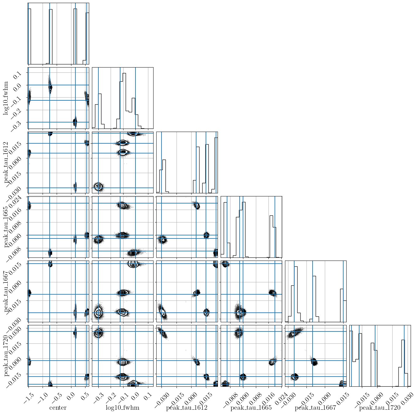
# Plot the marginalized posterior samples. One plot is created
# per component (named corner_0.png, corner_1.png, etc. in this example)
# and one plot is created for the component-combined posterior
# (named corner.png in this example). For simulated data, you can
# supply the truths dictionary to overplot the "true" values
model.plot_corner("corner.png", truths=truths)

# Get the posterior point estimate mean, standard deviation,
# and 68% highest density interval
summary = model.point_estimate(stats=["mean", "std", "hdi"], hdi_prob=0.68)
print(summary['center'])

Determining the optimal number of components

The Amoeba class is essentially a wrapper of many models, each with a different number of components. The same prior and likelihood distributions are assigned to each model. The initialization will look familiar:

from amoeba2.amoeba import Amoeba

# Initialize amoeba2
amoeba = Amoeba(max_n_gauss=10, verbose=True, seed=1234)

# Add priors
amoeba.set_prior("center", "normal", np.array([0.0, 1.0]))
amoeba.set_prior("log10_fwhm", "normal", np.array([0.0, 0.25]))
amoeba.set_prior("peak_tau", "normal", np.array([0.0, 0.01]))

# Add likelihood
amoeba.add_likelihood("normal")

# Add data
amoeba.set_data(data)

# models for each number of components are stored in this dictionary,
# which is indexed by the number of components
print(amoeba.models)
# So you could interact with individual models via
# amoeba.models[1].fit()

At this point there are two strategies for identifying the optimal number of components. Both will stop when the chain and component convergence checks pass, or when there are sampling divergences, or when the number of components exceeds max_n_gauss above, or when the BIC of the mean point estimate of the posterior samples increases twice in a row.

Otherwise, the difference is how amoeba2 decides how many components to try in successive iterations.

# fit_all() will start with 1 component and increment by one each time
# amoeba.fit_all(tune=1000, draws=1000, chains=8, cores=8)

# fit_best() will start with 1 component, and at each iteration it will try
# n_gauss set by the GMM prediction for the optimal number of components.
amoeba.fit_best(tune=1000, draws=1000, chains=8, cores=8)

The "best" model -- the first one to pass the convergence checks, or otherwise the one with the lowest BIC, is saved in amoeba.best_model.

print(amoeba.best_model.n_gauss)
# 4

posterior_predictive = amoeba.best_model.posterior_predictive_check(
    thin=50, plot_fname="posterior_predictive.png"
)
amoeba.best_model.plot_corner("corner.png", truths=truths)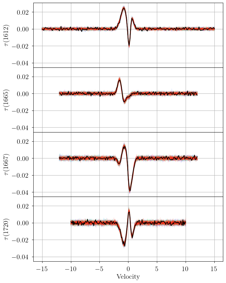

Known Issues

1. amoeba2 currently only implements fitting optical depth spectra, and not the more general case of optical depth and brightness temperature spectra as in the original amoeba.

Issues and Contributing

Anyone is welcome to submit issues or contribute to the development of this software via Github.

License and Copyright

Copyright (c) 2023 Trey Wenger

Permission is hereby granted, free of charge, to any person obtaining a copy of this software and associated documentation files (the "Software"), to deal in the Software without restriction, including without limitation the rights to use, copy, modify, merge, publish, distribute, sublicense, and/or sell copies of the Software, and to permit persons to whom the Software is furnished to do so, subject to the following conditions:

The above copyright notice and this permission notice shall be included in all copies or substantial portions of the Software.

THE SOFTWARE IS PROVIDED "AS IS", WITHOUT WARRANTY OF ANY KIND, EXPRESS OR IMPLIED, INCLUDING BUT NOT LIMITED TO THE WARRANTIES OF MERCHANTABILITY, FITNESS FOR A PARTICULAR PURPOSE AND NONINFRINGEMENT. IN NO EVENT SHALL THE AUTHORS OR COPYRIGHT HOLDERS BE LIABLE FOR ANY CLAIM, DAMAGES OR OTHER LIABILITY, WHETHER IN AN ACTION OF CONTRACT, TORT OR OTHERWISE, ARISING FROM, OUT OF OR IN CONNECTION WITH THE SOFTWARE OR THE USE OR OTHER DEALINGS IN THE SOFTWARE.