This report aims to provide a detailed analysis of the customer personality data set. Section 2 describes the methodology applied to explore the data set. The empirical results are presented in section 3. The main findings on clusters are discussed in section 4. The final section provides practical recommendations for the company to better serve consumers in each cluster.
The data is avaiable at customer-personality.csv file
We assume that web visits and purchase numbers in different channels are companies’ main concern as consumer behaviours, so we attempt to extract clusters from these features and categorize consumers via extracted labels.
To examine the predicted labels’ validity, we will use cluster outputs as dependent variable and others as independent variables to figure out if the clusters are well enough to epitomize different types of consumers. A simple supervised machine learning can deal with the validation. The conclusion is that the individual information (kids at home etc.) and consumption habits (meat consumption amounts etc.) can signify their consumer behaviours, bolstering the validity of clustering outputs and it’s also feasible to check decisive features to classify different types of consumers.
Aside from behaviour-related data, we also assume that remaining data, mainly consisting of consumer’s individual information and consumption habits, are reasonable source of customer segmentation. Given its multi-dimensionality, we need to deploy a dimension reduction strategy to overcome its complexity and discern pivotal features. PCA, ICA and FA are taken into considerations.
Compared to PCA and ICA, factor analysis can capture unique variance of specific and errors. It also retains a smaller dimension (8) than PCA (more than 10) while keeping a satisfactory explained variance. Likewise, Factor analysis is designed to project a high-dimension data to a lower vector space on account of feature’s specific variance and error. Compared to simple clustering, it gives an ordered attention to features that best discriminate the dataset. Thus, in contrast to unweighted clustering, FA can split the data more separately in the first several dimensions, leading to a more accurate categorization in theory.
This section will begin by presenting the K-means clustering with behaviour-related columns. After that, the K-means clustering with factor analysis will be presented.
We dropped the non-factorial categorical variables in consumer information (marital status etc.) and processed the factor analysis and clustering with remaining data. We matched the clustered output to consumer information and examined whether the labels accommodate to the categorical variables.
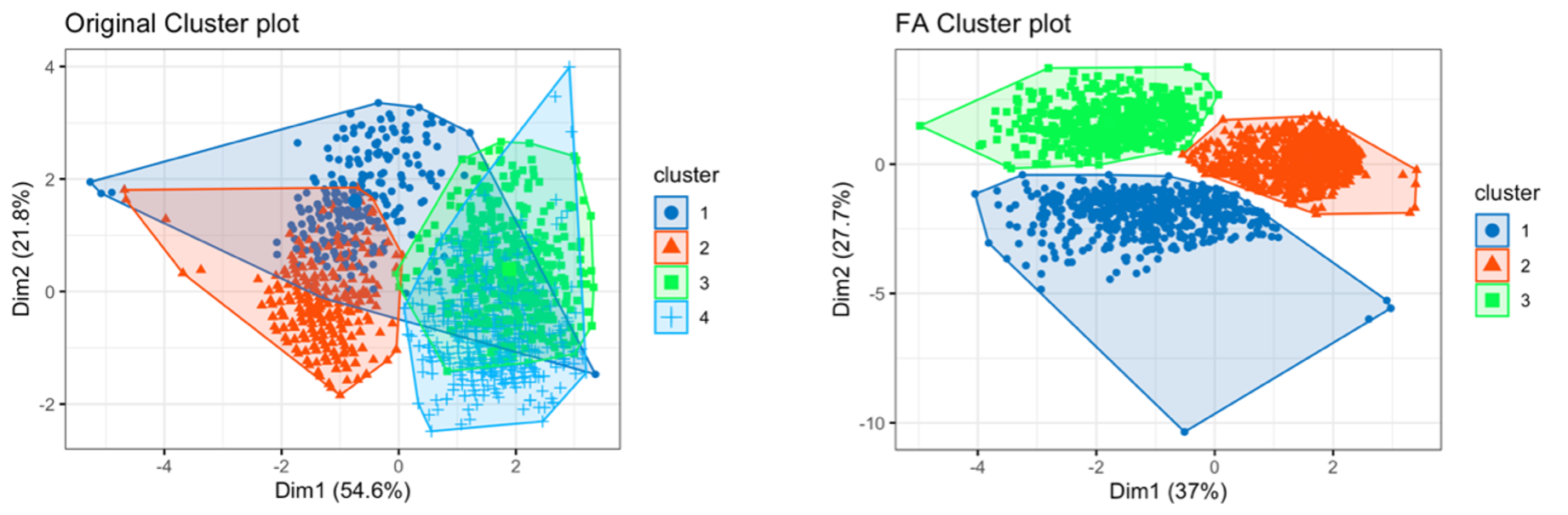
We drew the overlapping and distribution plot in first two dimensions when using different methods, compared their effect and evaluated two clustering methods.
This section will begin by presenting the K-means clustering with original data. After that, the K-means clustering with factor analysis will be presented.
Based on the populated elbow plot in R code, the point with significant drop in variance is when k = 4 from the range of 1 to 10. Hence, 4 is the chosen optimal cluster number.
Plot 1 - Distribution of Clusters
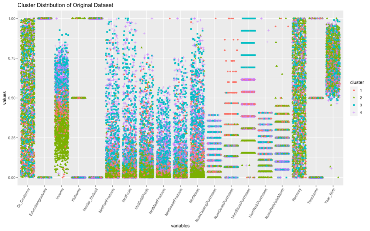
As can be seen from the distribution Plot 1, there are overlaps of observations from some features such as customer’s enrolment date and birth year, hence, no clear pattern is seen. However, a visible clear pattern is seen for other significant features such as income, amount spent on wine, fruits, meat, fish, sweet and gold in the last 2 years. Also, relationships can be identified from the dispersion patterns of purchases made through different channels.
Best model has a chi-square statistic is 7.182 on 7 degrees of freedom. The p-value for the chi-square test is 0.349 which is significantly larger than 0.05, indicating 8 factors have a good fit with the data set. Moreover, 8 factors have cumulative eigenvalues of 87%, confirming that the number of factors can properly explain the entire data set. Namely, first four factors contribute the most to the model according to the individual Eigen values (5.98, 1.78, 1.01, and 0.98). It is also clear that the model with rotation is better than the one without because a clear pattern in the factor loadings can be found in the former model to facilitate the interpretation of factors.
Plot 2 – Factor Analysis Loadings

Plot 2 describes the loadings for each Factor on different features. The variable income is mainly influenced by Factor 1, 2,3,6. Factor 2 has the most impact on Dt_customer. Recency is not largely determined by the any of factors in the model since it only has a loading of 0.108 on Factor 8. Features related to amount of purchase on different product categories including MntFruits. MntFishProducts and MntSweetProducts, are significantly influenced by Factor 1, while Factors 3 and 4 have significant impact on Mntwines (loading = 1.034) and MntGoldProds (loading = 0.973) respectively. Loading result shows similar partner on the number of purchases on different channels. NumDealsPurchases is mainly influenced by Factor 2 and 6. Factor 8 has the most impact on NumWebPurchases. NumCatalogPurchases are impacted by multiple factors, NumStorePurchases by Factor 5 and NumWebVisitsMonth by Factor 2 (loading = 0.862).
Plot 3 – Original Variables Distribution

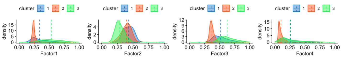
Elbow chart in R code indicates a cluster of three will be optimal in this case, given that it can explain more than 80% of the variance. Plot 3 describes clusters distribution based on different factors. Within Factor 1, cluster 1 and 2 distributed sparsely between 0.25 to 1 with Cluster 1 concentrate more on 0.125 to 0.75 and cluster 2 on 0.375 to 1, while Cluster 1 has least variance, concentrating on values around 0.25. Factor 2 saw different pattern that the variance among Clusters is small. cluster 3 have a lower value than cluster 1 and 2, Similar distribution has been observed on Factor 3, 4, 5, and 6 that Cluster 2 has the lowest value and the separation is very distinct. Factor 7, on the other hand, saw clear separation on Cluster 3 with a higher value. Lastly, Factor 8 observed the highest overall concentration with cluster 1 being higher on average than other clusters.
This section summaries findings based on cluster created by original data and factor analysis.
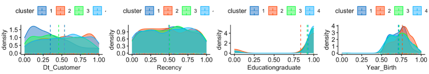
Plot 4 – Original Variables Distribution
 Plot 5 – Factor Analysis of Factors Distribution
Overall, similar patterns on average values of features for each cluster are observed on both clustering method with and without factor analysis. It is worth mentioning that Plot 4, 5 and 6 describes clusters created by factor analysis show clear distinction without any overlap while clusters created without factor analysis saw significantly overlap, indicating factor analysis perform well in dealing with nose data. On the other hand, even though there are difference in distribution in clusters created by these two methods, similar importance such as income, meat and sweat purchase amount can be discovered on both methods, indicating these features are determining variables. The following sections will elaborate on each clustering method.
Plot 6 – Factor Analysis and Original Data Clusters Distinction Distribution
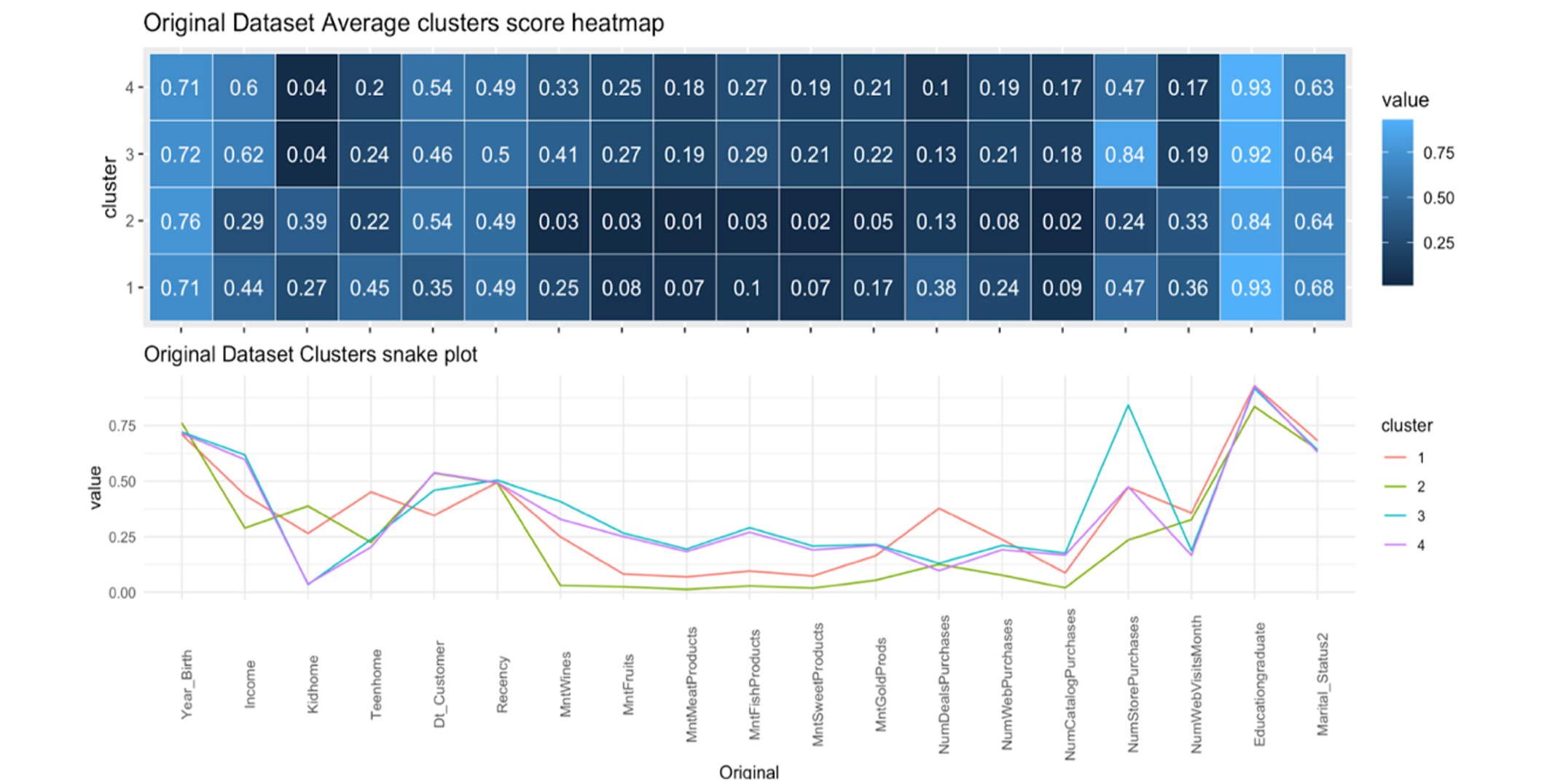
Plot 7 and 8 shows that purchasing behaviour of retail customers from four different clusters would vary according to the features of the individual. The fluctuation of the purchasing behaviour can be explained based on some significant demographic features and total amount purchased on products in that cluster.
Plot 7 – Original Data Cluster Mean & Snake Plot
Plot 8 – Factor Analysis Cluster Mean & Snake Plot
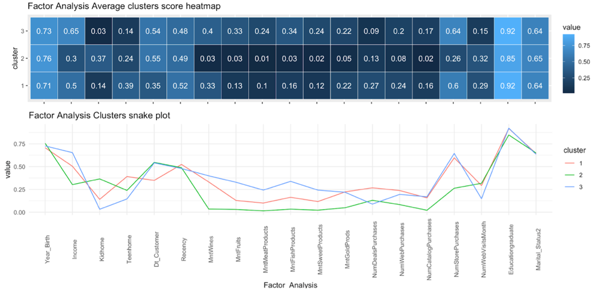
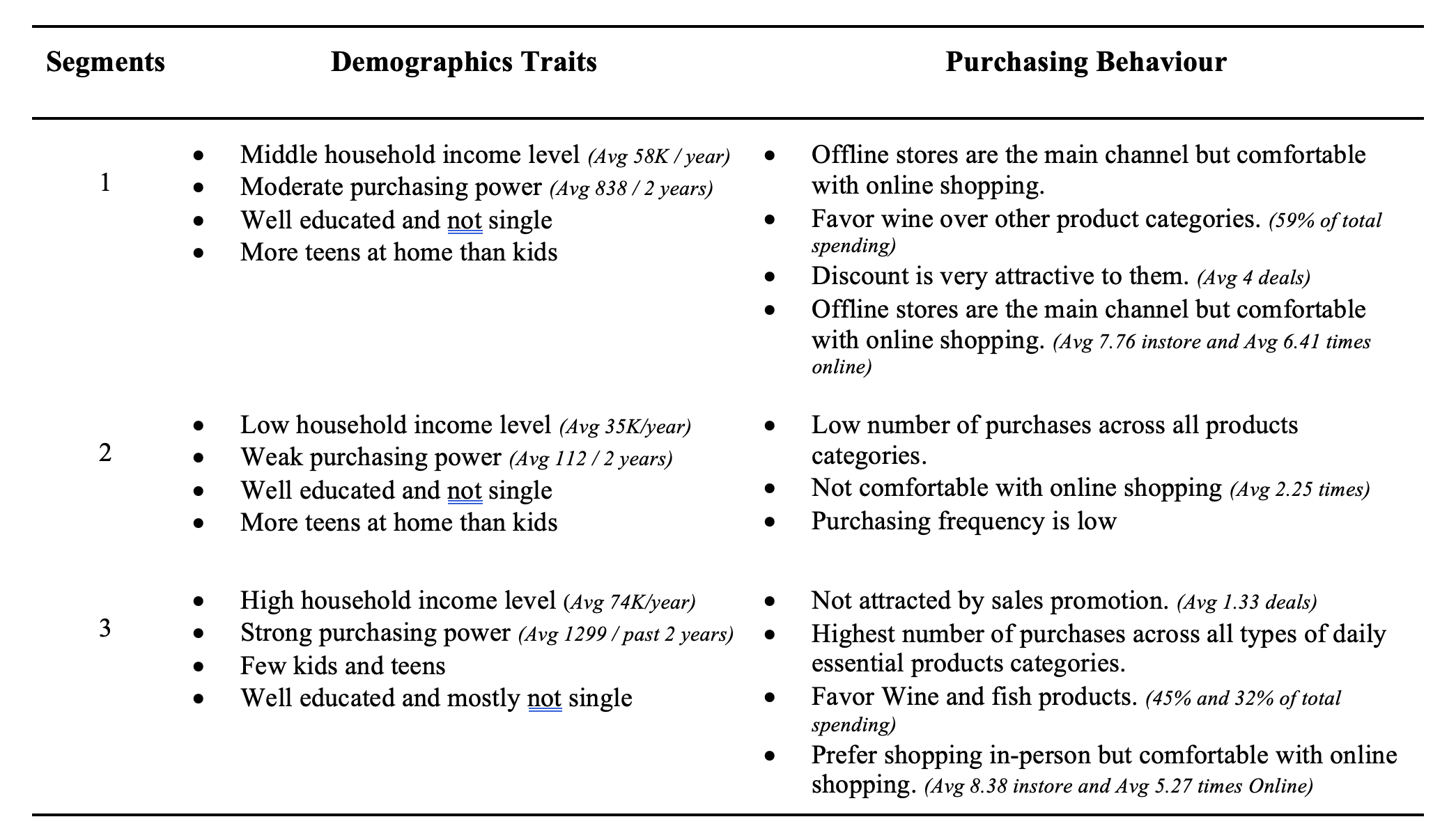
Based on the result from Factor analysis and K-means from Plot 8, findings were generated concerning each cluster:
Recommendation tailored to each cluster is provided to the company based on the finding and analysis from previous section.
Customer Segment 1
Cluster 1 has less monetary potential comparing to cluster 3; however, the company is advice to invest on this group of consumers accordingly. Frequent sales promotion, especially on wine, should be given to this segment, provided that discount is one of their purchase incentives. Since consumers in cluster 1 are comfortable with online shopping, digital campaigns via different channels featuring product discount should be created for them.
Customer Segment 2
The company is advised to not focus on this cluster of customers since analysis indicates it has the lowest monetary potential and contribution to the company. Any commercial initiates for this cluster would likely yield low return on investment.
Customer Segment 3
Building business strategies focusing on cluster 3 is recommended, given that consumers in this cluster have huge monetary value and they are active buyers. More specifically, high-end product segments, especially fish and wine, can be developed targeting this group of people, and exclusive in store shopping services can be provided, ensuring great customer experience. Marketing campaigns should also be created following same logic. Digital initiatives can also be experimented on this cluster since they are willing to shop online.