(1) Fit a decision tree to the training data with an optimal tree size determined by 5-fold cross-validation. Create a plot of the pruned tree and interpret the results. Compute the test error rate of the pruned tree.
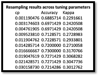
The optimal pruned tree is with the cp (alpha value ) of 0.01666667 and with train dataset of accuracy 0.7300000. For the test dataset of fitting to the decision tree, the test error is equal to 1- accuracy of test dataset, which is 0.2866667.
With using fancyRpartPlot from the rattle package, the plot of optimal pruned tree of train model is showing as below:
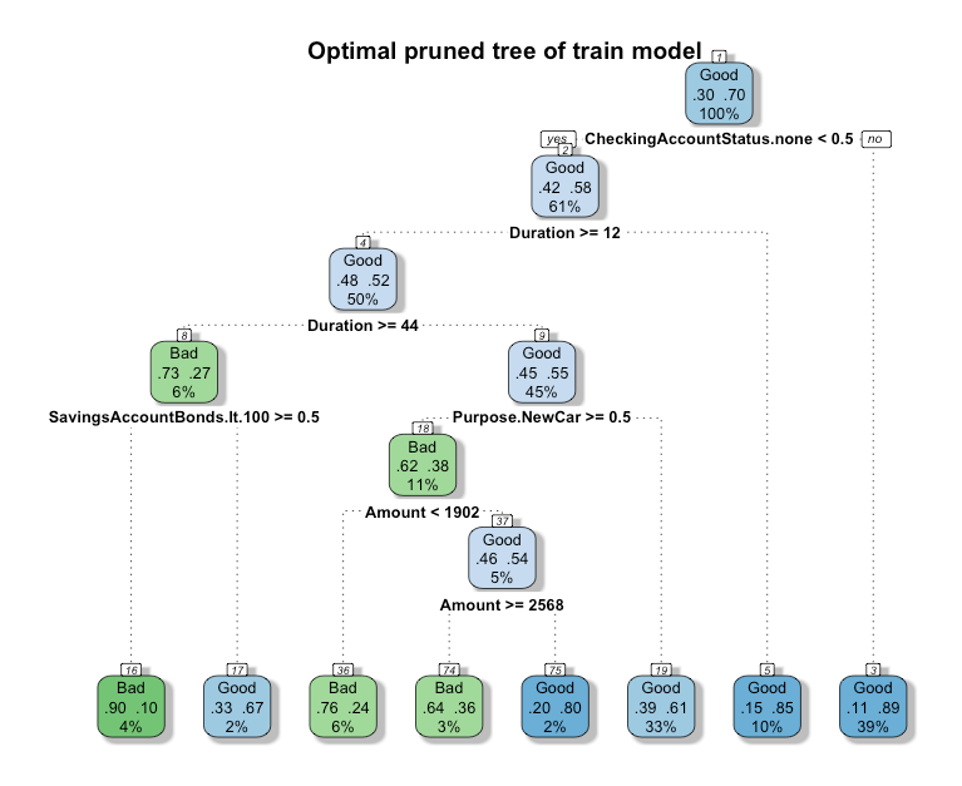
Observing from the figure, we can find that a total of 8 leaves and 5 variables, which is CheckingAccountStatus.none, Duration, Purpose.NewCar, SavingAccountBonds, and Amount, are used in our train model. It is worth noting that the two variables "CheckingAccountStatus.none" and "Duration" can already help us explain that the results of the Class "Good" for up to 49% of the overall data set. And the accuracy rate of deciding class = good can reach 85% and 89%, which means that the interpretability of these two variables is quite good.
The decision path of the train model is: when CheckingAccountStatus.none is greater than or equal to 0.5, it is judged as "Good", and if it is less than 0.5, it is judged by Duration. Then If the Duration of the data point is less than 12, it will be classified as "Good", if it is greater than or equal to 12, it will be set to judge in another range, or judged with other variables.
(2) Fit a random forest to the training data with the parameter of the number of features to create the splits tuned by 5-fold cross-validation. Set the number of trees to 1000. Compute the test error rate and comment on the results. Create a plot showing variable importance for the model with the tuned parameter and comment on the plot.
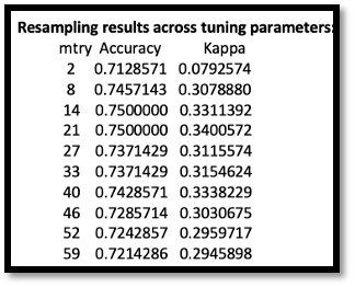
We have already known that mtry is the number of variables randomly sampled up at each split, with the output of different mtry, we could get the final value used for the train model was mtry = 14 with train set accuracy of 0.7500000. For the test dataset, the test error is equal to 1- accuracy and is equal to 0.25.
If we compare with the decision tree, we can find that the test error rate of random forest is lower than that of decision tree. This is because the random forest is an overall learning algorithm generated by using bagging and random feature sampling, so the result is less likely to overfit the train set, the generalization ability is stronger than that of the decision tree, and the prediction accuracy on the test set can be improved.
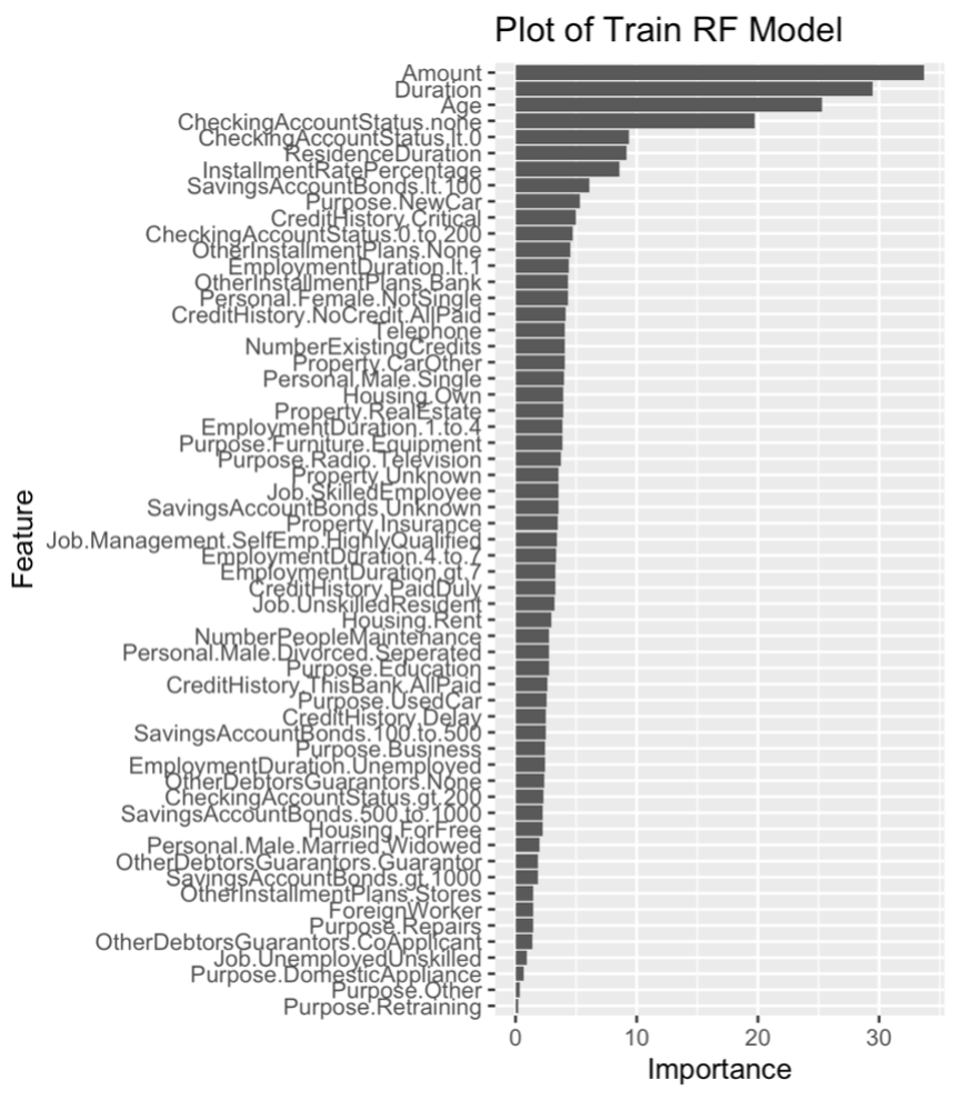
Now let's look at variable importance with the tuned parameters plotting for the train model:
In the R script, we use scale = FALSE to prevent scaling when plotting, so that the real value can be displayed. There are two measures of importance given for each variable in the random forest: Accuracy decreases and Gini impurity decreases. From the importance measured by these two values, it can be found that Amount, Duration, Age, CheckingAccountStatus.none, CheckingAccountStatus.lt.0, and ResidenceDuration are the top five important variables in order. Compared with the five variables in the decision tree, three variables (Duration, CheckingAccountStatus.none , and Amount ) all appear in the training model, indicating that they are all important. It can also be seen that the variavles of Propose relating has no significant effect on distinguishing class.
 We can observe from the figure that (1.) the ROC curve of Random Forest will be higher than that of decision tree, and the AUC of Random Forest is 0.756, which is better than the Decision Tree of 0.682. (2.) We find that ROC in Random Forest will be closer to a smooth curve; and Decision Tree has an obvious corner when FPR is equal to 0.2, which shows that the threshold point will greatly affect the accuracy rate of test set, and also shows that Random Forest has better generalization ability (because it is bagging sampling).
Simulate a three-class dataset with 50 observations in each class and two features. Make sure that this dataset is not linearly separable.

For information and comments, please see the r script for question 2, thank you.
(2) Split the dataset to a training set (50%) and a test set (50%). Train the support vector machine with a linear kernel, a polynomial kernel and an RBF kernel on the training data. The parameters associated with each model should be tuned by 5-fold cross-validation. Test the models on the test data and discuss the results.
For the linear kernel SVM:
The default setting of linear kernel SVM is holding a constant of cost = 1, which might not output the best optimal model. In this case, adding tuneGrid with different cost could solve the default issue. But after truning, we found that different costs will not bring better accuracy rate on train set. The optimal Cost = 0.4 with accuracy 0.5600000 on the train set, and all of the accuracy of costs are below 0.60(as shown in the figure below).

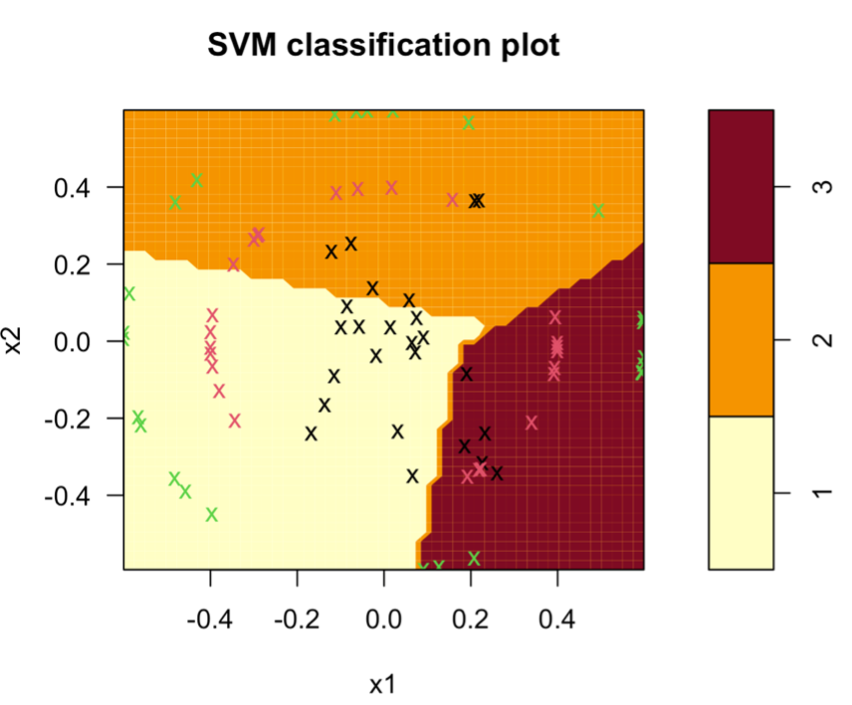
If we put it back in the test dataset for verification, we will find that its average accuracy is only 0.4133333, which shows that linear SVM is not suitable for distinguishing such datasets and will cause the model to overfit. If we take a closer look at Overall Statistics, we will also find that P-Value [Acc > NIR] : 0.09044. Represents no rejection: "The correct probability of picking a class at random" is not significantly different from the correct probability of using the model to classify. In short, Linear is not suitable for this kind of dataset distribution (the graph below also shows that its classification is quite bad).
For the polynomial kernel SVM and the RBF kernel SVM:
As for polynomial kernel, it can map data from low-dimensional space to high-dimensional space, but there are many parameters and a large amount of calculation. When running the code, the efficiency of Linear and RBF will be higher than that of polynomial. RBF can also map samples to high-dimensional space, but it requires fewer parameters than polynomial, and usually has good performance, so usually it is the default kernel function. Through the results in the table below:
we can find that both polynomial and RBF kernels have very accurate prediction capabilities on the test set, representing multi-dimensional space, and these two models can be well applied to classify labels. Their P-Value [Acc > NIR] are both rejecting hypothesis, and we can also see that the classification are very good (polynomial on the left and RBF on the right) from the distribution graph below.

It is worth noting that polynomial is insinuated in "limited dimensional space", while RBF is "infinite dimensional space". So once polynomial has been able to perfectly classify our simulated data set and the test set has a high accuracy rate, using RBF theoretically will not be much worse than the accuracy of polynomial, which is also explaining why the dataset on both polynomial and RBF kernel is over 90% accuracy on test set and similar (the size of the samples may cause fluctuations).
Download the newthyroid.txt data from moodle. This data contain measurements for normal patients and those with hyperthyroidism. The first variable class=n if a patient is normal and class=h if a patients suffers from hyperthyroidism. The rest variables feature1 to feature5 are some medical test measurements.
(1) Apply kNN and LDA to classify the newthyroid.txt data: randomly split the data to a training set (70%) and a test set (30%) and repeat the random split 10 times. For kNN, use 5-fold cross-validation to choose k from (3, 5, 7, 9, 11, 13, 15). Use AUC as the metric to choose k, i.e. choose k with the largest AUC. Record the 10 test AUC values of kNN and LDA in two vectors.
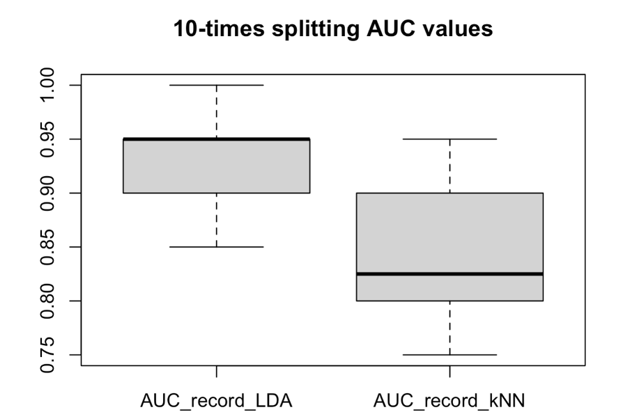
In order to fix the result each time, we discarded the original argument of time= 20 in createDataPartition. Instead, we wrote a for loop to record both train and test into two list with 10 times randomly spilts, and used the caret package to iterate the loop and record the AUC produced by method = “lda” and “knn”. It is worth noting that when creating a kNN model, with tuneGrid set to k from (3, 5, 7, 9, 11, 13, 15) to find the most good auc solution. We use list to record the auc results of each model, including AUC_record_kNN and AUC_record_LDA.
(3) What conclusions can you make from the classification results of kNN and LDA on the newthyroid.txt data?
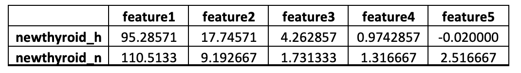
Before applying the model, we first separate the data sets with class = "h" and "n", and take the average value in each field, as shown in the table below, we can find that the average distribution between the two classes is very significant (To be more rigorous, we could also use ANOVA to obtain whether there is a significant difference).
From the box plot of question3(2), we can observe that whether it is kNN or LDA model, there is an average AUC on test set of more than 80%, which means that both models can identify different classes well, and the models are very good. However, there are still some differences:
- LDA is to find the best and single plane or line to classify h and n according to the sub-status of the data set; but the kNN model makes inne more inner, and the distance between outer and outer is farther. In this case , we have already known that the distribution of class h and class n has obvious differences, so whether it is LDA or kNN can make the model classification have a good performance
- In the kNN model, The k was choosing in the cross-validation in the training set, but this might not ne the optimal k in the testing set. This can also explain why in the plot of AUC_record_kNN the datapoints are more spreaded in the box (the variance is higher than LDA). It is believed that the LDA model will be more robust.
- The true classification boundary might be linear, kNN might be more flexible in non-linear separated classification. Finally, we also found that if we changed the seed, sometimes there would be obvious changes in the results. The reason may be that the number of samples is too small (the overall dataset has only 185 observations), but no matter how the random seed changes, both kNN and LDA can make the average AUC performance exceed 0.90, which means that both methods are good solutions.
Use this function to produce the training indexes for 10-fold cross-validation on the Ger- manCredit data. For information and comments, please see the r script for question 4, thank you.