Background Overview

When using deep learning or machine learning for classification, things are easiest if classes are “balanced” – that is, when the number of observations belonging to each of the classes are of the same order of magnitude. Unfortunately, this is often not the case.

Nevertheless, we want to create a model that helps the insurance provider target its investigation efforts. For this, we consider two options:

1. SMOTE: synthetically creating new data to make the dataset more balanced
2. Auto-Encoder: to represent “normal” (non- fraudulent) claims and applying it to distinguish fraudulent claims – a form of anomaly detection.

Data Source

1. The Insurance_claims.csv data is on google drive HERE
2. The dataset is abou car-insurance claims and to classify claims into fraudulent (1) and non- fraudulent (0).
3. There are more than 10,000 claims in the dataset, but only around 100 are fraudulent.

Description of the Data Features

Lexicon of the variables

Claimant- specific information

variables	explaination
PolicyholderNumber	Unique policy number for each policyholder
FirstPartyVehicleNumber	Vehicle number
PolicyholderOccupation	Occupation of the policyholder
FirstPolicySubscriptionDate	Subscription date
FirstPartyVehicleType	Type of vehicle (car, motorcycle, ...)
PolicyWasSubscribedOnInternet	1 if policy subscribed online; 0 otherwise
NumberOfPoliciesOfPolicyholder	Number of subscribed policies
FpVehicleAgeMonths	Age of car at time of incident (months)
PolicyHolderAge	Age of policyholder
FirstPartyLiability	Percentage of first party liability covered

Incident- specific information

variables	explaination
ThirdPartyVehicleNumber	Vehicle number of third party if applicable
InsurerNotes	Insurer notes about the incident (free text)
LossDate	Date of the covered incident
ClaimCause	Cause of the incident
ClaimInvolvedCovers	Policy covers used by the claimant
DamageImportance	Importance of damages as assessed by expert, in case assessment took place
ConnectionBetweenParties	Connection between parties if known
LossAndHolderPostCodeSame	1 if postcode of incident same as postcode of policyholder; 0 otherwise
EasinessToStage	Indicator of easiness to stage the accident (computed by insurance company)
ClaimWihoutIdentifiedThirdParty	1 if no other party involved; 0 otherwise
ClaimAmount	The amount of money claimed
LossHour	Hour of the incident
NumberOfBodilyInjuries	Number of injured persons in the incident
Fraud	1 in the case of fraud; 0 otherwise

plotting the variable of Fraud (1 and 0) of distribution after preprocessing

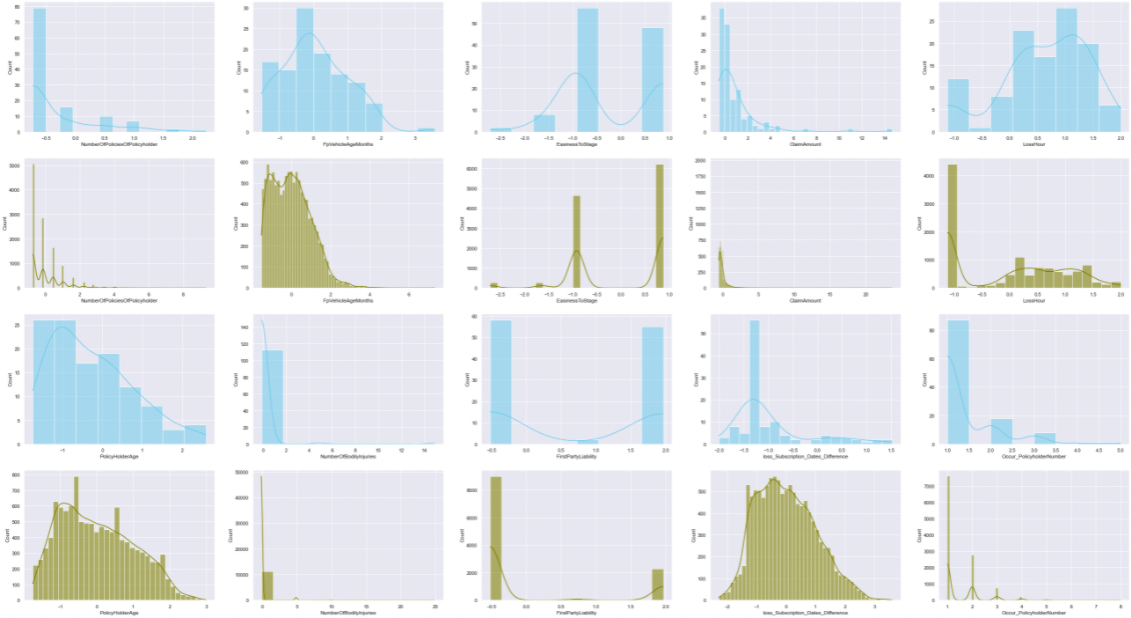
Note rthat we take a look at the scalar data (but not really apply the scalar here, we should apply after the split)

See all the features differences of 0 and 1 with the mean after preprocessing

Inside the DL_SMOTE&AutoEncoder.ipynb file...

1. would discuss why it is more difficult to find a good classifier on such a unbalanced dataset.
2. In particular, consider what happens when undetected fraudulent claims are very costly to the insurance company.

Benchmark model (without SMOTE or Auto-Encoder)

1. Would start by creating a neural network in TensorFlow and train it on the data.
2. Using training and validation sets, find a model with high accuracy,
3. The model is save as the original_turning_model.h5 file, and and evaluation is as below:

# evalute the model on test set
model_Q3.evaluate(X_test, Y_test)

91/91 [==============================] - 0s 870us/step - loss: 0.0455 - accuracy: 0.9899 [0.045471351593732834, 0.9899340271949768]

# get the AUC score
roc_auc_score(Y_test, Y_prob)

0.8869879576340862

# set treshold and get the final result    
threshold = 0.001
Y_predict = np.where(np.array(Y_prob)>=threshold, 1, 0)

# create confusion matrix 
cm = confusion_matrix(Y_test, Y_predict)
TN = cm[0][0]
FP = cm[0][1]
FN = cm[1][0]
TP = cm[1][1]
# print out the true positive and negative rate
print('true negative rate is ' + str(TN/(FP+TN)))
print('true positive rate is ' + str(TP/(TP+FN)))

true negative rate is 0.28225806451612906 true positive rate is 0.9655172413793104

SMOTE approach to simulate the data

1. Create new (synthetic) data points representing fraudulent claims and remove some of the non-fraudulent claims.
2. This will allow us to create a more balanced dataset. The state-of-the-art method we apply is SMOTE (Synthetic Minority Oversampling Technique).
3. We furher use the tuner to get the best hyperparameters
4. Create a new neural network and train it on the enhanced dataset, saved as the smote_turning_model.h5 file

# visualise the lost 
plt.plot(log_2.history['loss'],label = "training loss")
plt.plot(log_2.history['val_loss'], label = "validation loss")
plt.legend()
plt.show()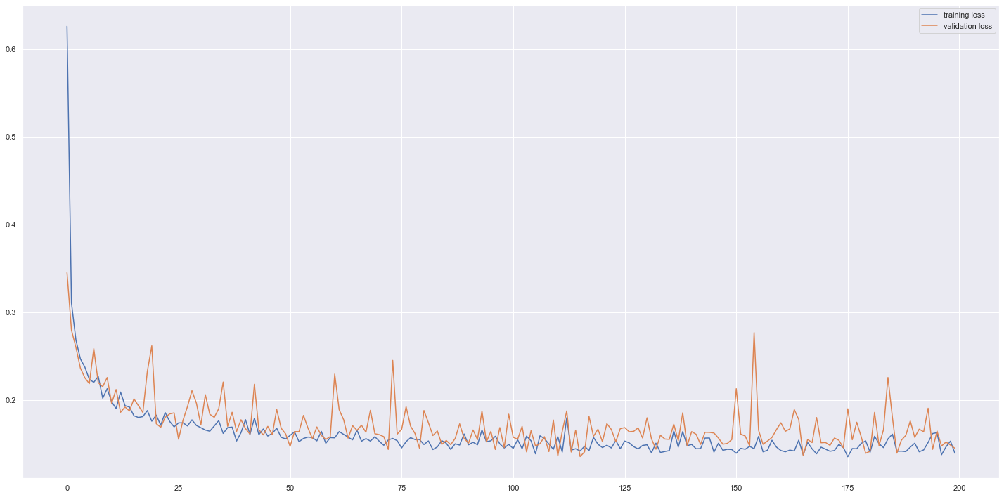

# evalute the model on test set
model_Q5.evaluate(X_test, Y_test)

91/91 [==============================] - 0s 1ms/step - loss: 0.1723 - accuracy: 0.9611 - tp: 8.0000 - auc: 0.7660 [0.1722506880760193, 0.96112459897995, 8.0, 0.7659597396850586]

# make prediction on test set
Y_prob_2 = model_Q5.predict(X_test)
Y_prob_2 = Y_prob_2.reshape(-1,)
Y_prob_2 = [ y for y in Y_prob_2]

# get the AUC score
roc_auc_score(Y_test, Y_prob_2)

0.8341454272863569

# set treshold and get the final result 
# the treashold was found by observing the distribution of probability of Fradulent and Non-Fradulent
threshold = 0.003
Y_predict_2 = np.where(np.array(Y_prob_2)>=threshold, 1, 0)

# create confusion matrix 
cm = confusion_matrix(Y_test, Y_predict_2)
TN = cm[0][0]
FP = cm[0][1]
FN = cm[1][0]
TP = cm[1][1]

# print out the true positive and negative rate
print('True Negative rate (Sensitivity)' + str(TN/(FP+TN)))
print('True Positive rate (Specificity)' + str(TP/(TP+FN)))

True Negative rate (Sensitivity)0.7738429172510519
True Positive rate (Specificity)0.8275862068965517

A combination of SMOTE oversampling and undersampling methods is applied to create a balance of 50:50 for both fraud and non-fraud classes. The concept is because we apply a modest amount of oversampling to the minority class, which improves the bias to the minority class instances, whilst we also perform a modest amount of undersampling on the majority class to reduce the bias on the majority class instances. As we performed both SMOTE and undersampling, the total number of instances of synthesized dataset is close to that of the original dataset. By doing this, we could improve performance in comparison to the methods being performed in isolation.

After applying smote, the accuracy rate and auc are expected to drop and the gap between true positive and true nagative are also expected to narrow, compared with the original_turning_model.h5, because metrics are now indicative and algorithm has sufficient look at the underlying class and treat all observation of fradulent and non-fraudulent the same. Furthermore, even with balanced data, it is impossible to achieve a 99% true positive rate in real life. The actual outcome matched with previous expectation with a accuracy rate of 0.9611, auc 0.8341 and true positive rate and true negative rate

The smote_turning_model.h5 model is doing better on predicting fraudulent; however, the limitation on the smote and under-sampling is that it generates new data set based on the characters of the current fraudulent cases which might not be representative for all the fraudulent characteristics and therefore the prediction is difficult to reach a very good level such as above 95%.

Auto-Encoder approach to learn what "normal" (non-fraudulent) data "looks like."

1. Using the original data, create a training and set that contains only non-fraudulent claims, as well as validation and test sets that contain non-fraudulent and fraudulent claims and spread fraudulent claims evenly.
2. Using TensorFlow, create an autoencoder, ensuring that the middle hidden layer has fewer neurons than input features has.
3. Use training and validation sets to find a model that represents its input data well.
4. The model is saved as the autoencoding_turning_model.h5 file

X_test_pred = model.predict(X_test)
X_test_loss = tf.keras.losses.MeanAbsoluteError(reduction=tf.keras.losses.Reduction.NONE)(
    X_test, X_test_pred).numpy()
roc_score=roc_auc_score(y_test,X_test_loss)
roc_score

0.7244828683568474

fig=plt.figure(figsize=(15,5))
fig.add_subplot(111)
plt.xticks(np.linspace(0,1,21,endpoint=True),rotation=90)
sns.histplot(x=X_test_loss,y=y_test.squeeze(),hue=y_test)
plt.tight_layout()
plt.show()

threshold = 0.15
Y_predict = np.where(np.array(X_test_loss)>=threshold, 1, 0)
cm = confusion_matrix(y_test, Y_predict)
TN = cm[0][0]
FP = cm[0][1]
FN = cm[1][0]
TP = cm[1][1]
# print out the true positive and negative rate
print('true negative rate is ' + str(TN/(FP+TN)))
print('true positive rate is ' + str(TP/(TP+FN)))

true negative rate is 0.6435239206534422
true positive rate is 0.6181818181818182

We built a 5-layer autoencoder since it can keep majority of information in dataset and not too complex. Numbers of neurons in each hidden layer are tuned by Hyperband. With regard to other hyperparameter, we considered Adam weight decay optimizer, cosine annealing learning rate scheduler and loss function of MSE. This model obtained a AUC above 0.7 on validation set.

We have used HPtuner to choose best combination of neuron numbers in different hidden layers. The issue was, we found different outputs which can obtain a 10% difference in AUC, when running same codes in different laptops, even in the same device different times. Our solution is to not clear session, fit same model repeatedly and save the model with highest AUC. In this case, we reached AUC at 0.76 with validation data and 0.72 at test data. In general, autoencoder can usually reach above 0.7 with tuned models.

Randomness problem: The ROC solution is not the same every time. After our observation, we found that Loss will be inherited according to the log after the last run. But we still can't solve this problem after we have fixed the seed.

We can use our model to predict own dataset and examine sample wise error. Then we choose a threshold to determine which sample should be categorized into fraudulence. If error of a sample is larger than this threshold, then it should be deemed as fraudulence. Since it’s vital for insurance firms to discern positive samples correctly, we should choose a threshold with high true positive rate. We can see that autoencoder can reach AUC level of approximately 0.75, which means that it performs better than just tuning hyperparameters on original dataset, but its accuracy is not better than smote and down-sampling.

comparsion of different model

Model	Accuracy Score	AUC Score
original_turning_model	0.9899340271949768	0.8869879576340862
smote_turning_model	0.96112459897995	0.8341454272863569
autoencoding_turning_model	NA	0.7244828683568474
logistic_regression_model	0.9129451667608819	0.8806937519889678

Keep track of the accuracy and AUC on a test set made from original data only.

Above table summarizes the Accuracy and AUC scores of individual models we built including two neural network models from original_turning_model and smote_turning_model, autoencoder classifier and logistic regression. However, accuracy score is not applicable for autoencoder classifier, hence, we will make comparison of models based on AUC scores obtained.

Accuracy & AUC Scores Comparison:

1. original_turning_model vs logistic_regression_model

Neural network in original_turning_model has highest accuracy and AUC among all models but this does not mean that the model has actually outperformed logistic regression due to accuracy paradox. This is due to the neural network in original_turning_model is built on original imbalanced data whereby non-fraud falls under the majority class so the prediction of model is bias towards the non-fraud class of the dataset. The model will tends to learn well on non-fraud class and predict non-fraud class to achieve high accuracy score.

2. smote_turning_model vs logistic_regression_model

Neural network in smote_turning_model has slightly underperformed as expected when compared to the first neural network built in original_turning_model. This model is built after adjusting for imbalanced classes and it has proven to be outperform the logistic regression with higher accuracy and AUC score. Neural network provides more flexbility as the network size can be restricted by decreasing the number of variables and hidden neurons. Network can also be pruned after training. It is a nonlinear generalizations of logistic regression, so neural network is more powerful but more computationally expensive when compared to logistic regression that is much simple model.

3. autoencoding_turning_model vs Llogistic_regression_model

The approach for autencoder classifier is quite different from all other models that we have built, it acts as an extreme rare-event classfier for anomaly detection directly based on original imbalanced data. We observed an improvement in AUC score when compared to logistic regression. Autoencoder performs feature extraction and captures the efficient coding of the input data and projects it into lower dimension. For input data having a lot of input features as in our case of 61 features, it’s proven that model performance is better when we choose to project the data into lower dimensions and use the features for supervised learning task like insurance claim fraud detecton.

Does the model allow to answer a customer who asks, "why am I being investigated"?

Yes. It gives true postive rate of 0.996 and false positive rate of 0.257. However, the false positive rate is not very low that means authentic insurance claims could be potentially flagged out and misclassified as fraud claims. This creates unhappy customers who may leave and never return due to they are innocent after investigations. This creates a negative reputation. In general, although logistic regression is not the best model among all others machine learning models demonstrated here but it provides high interpretability of model parameters and has less complex model structure. In this case, it provides reasonable accuracy score of 73.48%, indicating a good model. It is more suitable for smaller and less complex dataset with lesser features.

Conclusion: Transparency of deep learning approaches

What’s the problem of using a neural network to a fraud:

1. Variable cannot be explained: because the neural network has many layers, and the layers are complicated. Compared with other regression methods, these variables cannot be explained, nor can they remind insurance companies which parts to focus on preventing in the early stage, and cannot solve the problem of fraud fundamentally or traceably.
2. Long operation time: When adding a new dataset, the model needs to be retrained. At present, the variables and datasets of the model are not too large and complex, but if there are many variables and datasets, compared with other regression models, it will take a lot of computing power and time to train new models.
3. Ensure that the TPR is high enough: In order to ensure that the insurance company will not be fraudulent, it will try to increase the True Positive Rate. This may cause the review before allowing insurance to be too strict, resulting in the sacrifice of reasonable claims and legal risks.
4. The model is becoming more and more difficult to learn: If the fraudster collects the claim data and his/her tech ability is good enough, he may be able to imitate deep learning and apply it to fraud to avoid it, or the model may change due to the change of features over time. The accuracy is getting lower and lower and would be also hard for model learning.
5. The problem of false negatives: Now the investigation results are actually not mature enough, and many frauds have not been completely eliminated or detected, so many cases of actual frauds have not been detected, which is the so-called fake negative. Therefore, the proportion of the dataset causing fraud in the data is very small. It may cause the features to be not obvious enough and the accuracy of the model to be poor, and the TPR to be not high enough, so if you want to achieve a very low fake negative rate, you will need to sacrifice a lot of revenue, which is not the most optimal solution.

Alternatives (more interpretability and transparency):
The following methods can directly explain the features that the model focuses on, and there are many improvements in interpretability and transparency:

1. Linear Regression: The advantage is that the model is intuitive and does not need to be trained first. The most important thing is that the computing power and time do not need too much, and the Variable can be explained. But the disadvantage is that we cannot do binary output (or categories output)
2. Logistics Regression: It can do binary or categorical (if having different thresholds) output, which makes up for the shortcomings of Linear Regression. We can observe the Logistic Regression in question 10 to understand the difference with the neural network. But the point is that many Features will not be detected or sacrifice some important information after preprocessing.
3. Decision Tree and Random Forest: The model accuracy may be more accurate than that of Logistics Regression or Linear Regression, and gini desreasing and accuracy desreasing can be used to distinguish Variables Importances, and the interpretability is also quite high.

Techniques learned in other courses that can be applied to the above methods:

1. NLP: Sentiment analysis can be used to analyze positive and negative sentiment, or it can be classified as new features by word group classification. Please note that we dropped the InsurerNotes’ columns in the previous data preprocessing, but if NLP can be used, it will be a good application
2. PCA: It can prevent too many dimensions from overfitting, but the disadvantage is the same as the neural network: once PCA is used, it may not be able to fully explain the importance of Variables