This file was generated using this jupyter notebook and code for the images used in this report can be found in the same.
The goals / steps of this project are the following:
- Perform a Histogram of Oriented Gradients (HOG) feature extraction on a labeled training set of images and train a classifier Linear SVM classifier.
- Optionally, you apply color transform and append binned color features, to HOG feature vector.
- Train a classifier to disinguish between car and non-car images
- Implement a sliding-window technique and use your trained classifier to search for vehicles in images.
- Run vehicle detection pipeline on a video stream and create a heat map of recurring detections frame by frame to reject outliers and follow detected vehicles.
- Estimate a bounding box for vehicles detected.
The jupyter notebook containing code for model training can be found here.
The code for HOG feature extraction can be found in ./utils/featureExtraction.py.
I started by reading in all the vehicle and non-vehicle images. Here is an example of one of each of the vehicle and non-vehicle classes:

I then explored different color spaces and different skimage.hog() parameters (orientations, pixels_per_cell, and cells_per_block). I grabbed random images from each of the two classes and displayed them to get a feel for what the skimage.hog() output looks like.
Here is an example using the YCrCb color space and HOG parameters of orientations=8, pixels_per_cell=(8, 8) and cells_per_block=(2, 2):

I tried various combinations of color spaces and parameters before finally settling with following:
color_space = 'YCrCb'
spatial_size = (32, 32)
hist_bins = 32
orient = 9
pix_per_cell = 8
cell_per_block = 2
hog_channel = 'ALL'
spatial_feat = True
hist_feat = True
hog_feat = True
Increasing the orientation enhanced the accuarcy of the finally trained classifier, but increased the time required for computation.
The color_space was decided by training a classifier on different color spaces for spatial features, and YCrCb performed better than RGB, HLS, and HSV.
The images were fliped and added back to the directory containing original images as an augmentation step.
The train_test_split from sklearn.model_selection was used to randomized the data and make a 80-20% train-test split. The split was made so as to keep the ratio of vehicles and non-vehicles similar.
The extracted features where fed to LinearSVC model of sklearn with default setting of square-hinged loss function and l2 normalization. The trained model had accuracy of 99.47% on test dataset. The SVC with rbf kernel performed better with accuracy of 99.78% as compared to the LinearSVC but was very slow in predicting labels and hence was discarded.
The trained model along with the parameters used for training were written to a pickle file to be further used by vehicle detection pipeline.
** Model training code can be found here. **
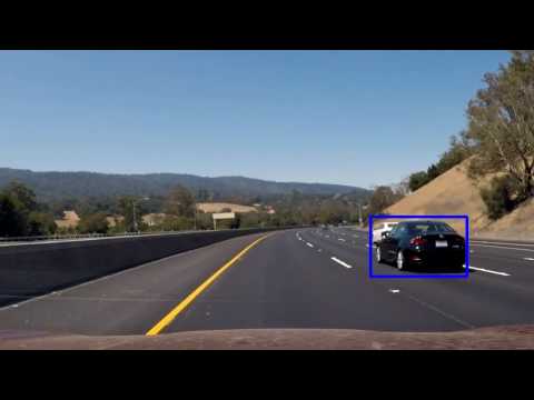
A single function, find_cars in ./utils/featureExtraction.py, is used to extract features using hog sub-sampling and make predictions. The hog sub-sampling helps to reduce calculation time for finding HOG features and thus provided higher throughput rate. A sample output from the same is shown below.
Code with multi-scale window search and heatmap to reduce false positives have been implemented in the class VehicleDetector in ./utils/vehicle_detector.py and is discussed in upcoming sections.

The scale for the multi-window search and overlap to be considered was decided emperically.
The multi-scale window approach prevents calculation of feature vectors for the complete image and thus helps in speeding up the process. The following scales were emperically decided each having a overlap of 75% (decided by cells_per_step which is set as 2):
Scale 1:
ystart = 380
ystop = 480
scale = 1
Scale 2:
ystart = 400
ystop = 600
scale = 1.5
Scale 3:
ystart = 500
ystop = 700
scale = 2.5
The figure below shows the multiple scales under consideration overlapped on image.

Falsely detected patch were explicitly used to create a negative example added to training set. The false positives were avoided by using wrongly classified examples and adding it to the training dataset.
Using YCrCb color space, the number of false positives were stemmed.
I recorded the positions of positive detections in each frame of the video. From the positive detections I created a heatmap and then thresholded that map to identify vehicle positions. I then used scipy.ndimage.measurements.label() to identify individual blobs in the heatmap. I then assumed each blob corresponded to a vehicle. I constructed bounding boxes to cover the area of each blob detected.

The search was optimized by processing complete frames only once every 10 frames, and by having a restricted search in the remaining frames. The restricted search is performed by appending 50 pixel to the heatmap found in last three frames. Look at the implementation of find_cars method of VehicleDetector in ./utils/vehicle_detector.py.

The youtube video of the final implementation can be accessed by clicking the following image link.
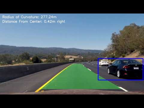
The youtube video of the opional implementation of simultaneous vechicle and lane detection can be accessed by clicking the following image link. The code for the same can be accessed here.
A neural network based model might provided better results for the classification for vehicles. Also, U-Net Segmentation might provided superior results as compared to window-based search approach.
The developed pipeline may possibly fail in varied lighting and illumination conditions. Also, the multi-window search may be optimized further for better speed and accuracy.
@book{binnani2019vision,
  title={Vision-based Autonomous Driving},
  author={Binnani, Sumit},
  year={2019},
  publisher={University of California, San Diego}
}