Stock Analysis

Package for making elements of technical analysis of a stock easier from the book Hands-On Data Analysis with Pandas. This package is meant to be a starting point for you to develop your own. As such, all the instructions for installing/setup will be assuming you will continue to develop on your end.

Setup

# should install requirements.txt packages
$ pip3 install -e stock-analysis # path to top level where setup.py is

# if not, install them explicitly
$ pip3 install -r requirements.txt

Usage

This section will show some of the functionality of each class; however, it is by no means exhaustive.

Getting data

from stock_analysis import StockReader

reader = StockReader('2017-01-01', '2018-12-31')

# get bitcoin data in USD
bitcoin = reader.get_bitcoin_data('USD')

# get faang data
fb, aapl, amzn, nflx, goog = (
    reader.get_ticker_data(ticker)
    for ticker in ['META', 'AAPL', 'AMZN', 'NFLX', 'GOOG']
)

# get S&P 500 data
sp = reader.get_index_data('S&P 500')

Grouping data

from stock_analysis.utils import group_stocks, describe_group

faang = group_stocks(
    {
        'Facebook': fb,
        'Apple': aapl,
        'Amazon': amzn,
        'Netflix': nflx,
        'Google': goog
    }
)

# describe the group
describe_group(faang)

Building a portfolio

Groups assets by date and sums columns to build a portfolio.

from stock_analysis.utils import make_portfolio

faang_portfolio = make_portfolio(faang)

Visualizing data

Be sure to check out the other methods here for different plot types, reference lines, shaded regions, and more!

Single asset

Evolution over time:

import matplotlib.pyplot as plt
from stock_analysis import StockVisualizer

netflix_viz = StockVisualizer(nflx)

ax = netflix_viz.evolution_over_time(
    'close',
    figsize=(10, 4),
    legend=False,
    title='Netflix closing price over time'
)
netflix_viz.add_reference_line(
    ax,
    x=nflx.high.idxmax(),
    color='k',
    linestyle=':',
    label=f'highest value ({nflx.high.idxmax():%b %d})',
    alpha=0.5
)
ax.set_ylabel('price ($)')
plt.show()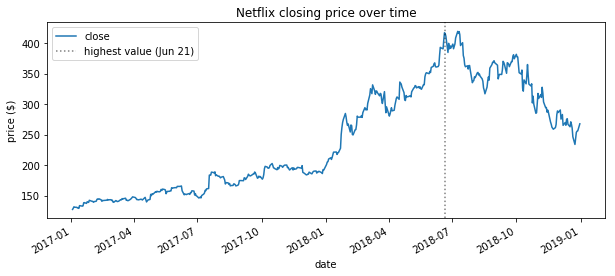

After hours trades:

netflix_viz.after_hours_trades()
plt.show()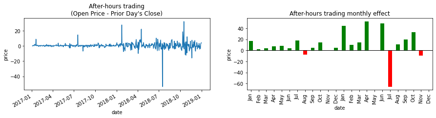

Differential in closing price versus another asset:

netflix_viz.fill_between_other(fb)
plt.show()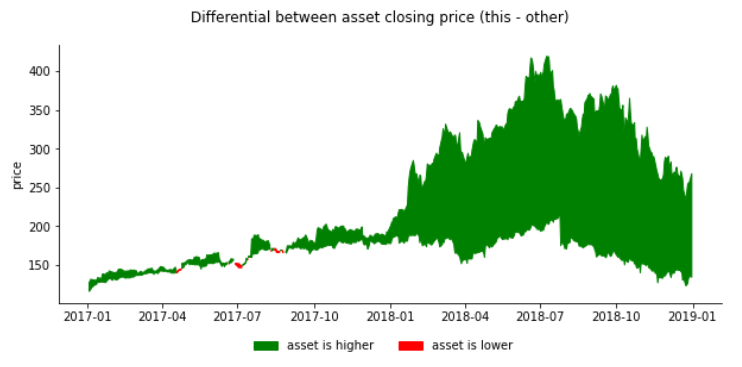

Candlestick plots with resampling (uses mplfinance):

netflix_viz.candlestick(resample='2W', volume=True, xrotation=90, datetime_format='%Y-%b -')

Note: run help() on StockVisualizer for more visualizations

Asset groups

Correlation heatmap:

from stock_analysis import AssetGroupVisualizer

faang_viz = AssetGroupVisualizer(faang)
faang_viz.heatmap(True)

Note: run help() on AssetGroupVisualizer for more visualizations. This object has many of the visualizations of the StockVisualizer class.

Analyzing data

Below are a few of the metrics you can calculate.

Single asset

from stock_analysis import StockAnalyzer

nflx_analyzer = StockAnalyzer(nflx)
nflx_analyzer.annualized_volatility()

Asset group

Methods of the StockAnalyzer class can be accessed by name with the AssetGroupAnalyzer class's analyze() method.

from stock_analysis import AssetGroupAnalyzer

faang_analyzer = AssetGroupAnalyzer(faang)
faang_analyzer.analyze('annualized_volatility')

faang_analyzer.analyze('beta', index=sp)

Modeling

from stock_analysis import StockModeler

Time series decomposition

decomposition = StockModeler.decompose(nflx, 20)
fig = decomposition.plot()
plt.show()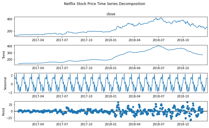

ARIMA

Build the model:

arima_model = StockModeler.arima(nflx, ar=10, i=1, ma=5)

Check the residuals:

StockModeler.plot_residuals(arima_model)
plt.show()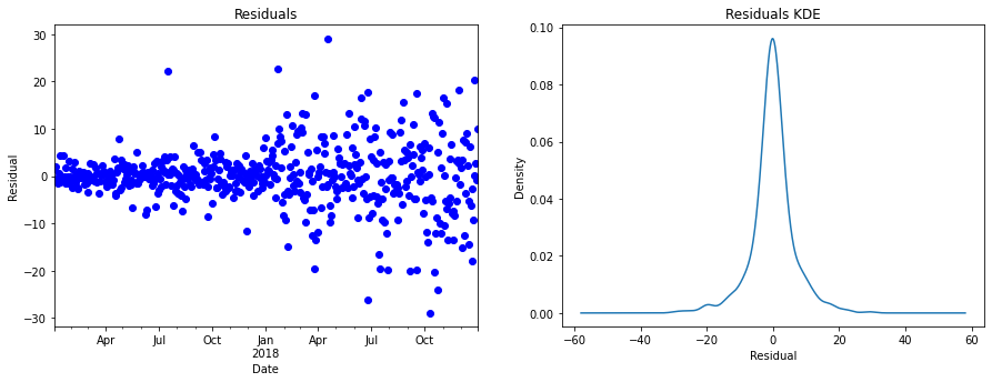

Plot the predictions:

arima_ax = StockModeler.arima_predictions(
    nflx, arima_model,
    start='2019-01-01', end='2019-01-07',
    title='ARIMA'
)
plt.show()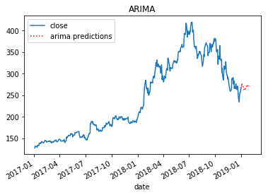

Linear regression

Build the model:

X, Y, lm = StockModeler.regression(nflx)

Check the residuals:

StockModeler.plot_residuals(lm)
plt.show()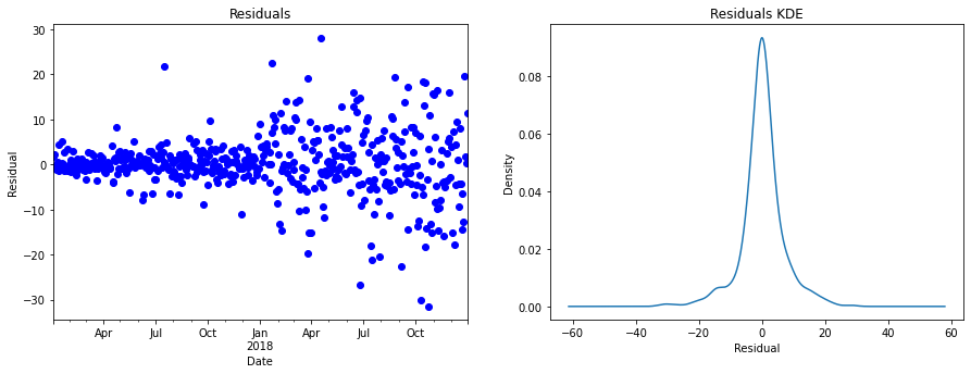

Plot the predictions:

linear_reg = StockModeler.regression_predictions(
    nflx, lm,
    start='2019-01-01', end='2019-01-07',
    title='Linear Regression'
)
plt.show()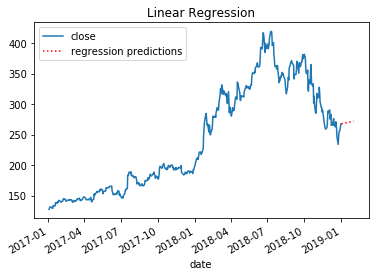

---

About the Author

Stefanie Molin (@stefmolin) is a software engineer and data scientist at Bloomberg in New York City, where she tackles tough problems in information security, particularly those revolving around data wrangling/visualization, building tools for gathering data, and knowledge sharing. She is also the author of Hands-On Data Analysis with Pandas, which is currently in its second edition and has been translated into Korean. She holds a bachelor’s of science degree in operations research from Columbia University's Fu Foundation School of Engineering and Applied Science, as well as a master’s degree in computer science, with a specialization in machine learning, from Georgia Tech. In her free time, she enjoys traveling the world, inventing new recipes, and learning new languages spoken among both people and computers.