This dataset contains 8732 sound excerpts (<=4s) of urban sounds from 10 classes: air_conditioner, car_horn, children_playing, dog_bark, drilling, enginge_idling, gun_shot, jackhammer, siren, and street_music.
This sound classification challenge contains 5435 training samples with labels and 3297 unlabelled test samples. This classification challenge is hosted on Analytics Vidhya which can be found here.
Amplitude is the size of vibration and it determines how loud a sound is. Frequency is the speed of vibration and it describes the pitch of the sound.
The audio quality can be measured using bit rate and sample rate. Bit Rate is measured in Kilo-bits-per-sec and it is the number of bit encoded in a second of audio. A lower bit-rate would mean lower sound quality and lower file size. Sample Rate is measured in Hertz and it defines how many times per second a sound is sampled. Sampling is the reduction of a continious time signal to a discrete time signal. A sampler extracts samples from a continious time signals. So if an audio has a sample rate of 44100 Hz, it means that each second is broken down into 44100 parts and values at those timestamps are stored.
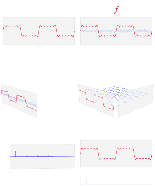
The fast fourier transform algorithm computes the discrete fourier transform (DFT) of an audio signal. It basically converts the audio from time domain to frequency domain. A time-domain graph shows how a signal changes over time, whereas a frequency-domain graph shows how much of the signal lies within each given frequency band over a range of frequencies.
A specrogram is a heatmap where the X-axis represents the time, Y-axis represents the frequency, with lower frequency at the bottom and the color determines the amplitude (how loud the sound is). So it basically shows how loud a particular frequency is at a particular time.
First, since the labels for test data weren't available, the training data was split into 80% training set and 20% validation set with equal proportions of data in each class. After splitting, the training set had 4350 samples and validation set had 1085 audio samples. 3 different models were trained on this dataset. Let's go through each of them.
When we read the data using librosa, we get a time series data with the default sampling rate of 22050, which means for every second, we have 22050 data points available. For this dataset, the data was read with the default sampling rate and then each audio sample was made to be of a fixed length of 4 seconds by either adding padding or trimming from the end.
This means that we have 88200 data points for each sample. This data was used for training an Artificial neural network. Since the number of features is nearly 20 times the number of samples, the model was expected to perform poorly but it was interesting to know the drawbacks of directly training on the time series data. Once the model was trained, the predictions were submitted on Analytics Vidhya which gave us the accuracy score.
Here are the results obtained:
| ANN | Training Set | Validation Set | Test Set |
|---|---|---|---|
| Accuracy | 96.67% | 19.26% | 17.44% |
| Loss | 0.2134 | 7.4628 | Not Available |
The time series data used for training the Artificial Neural Networkis not how humans perceive sound. So we first decompose the audio into different frequencies by using fourier transform and convert the frequency to mel scale which is how humans perceive sound. The amplitude is also converted to decibel which is also how humans perceive sound. Then, we get the spectrogram images of each audio whcih will be used to train our model. This conversion provides two benefits: it represents how humans perceive sound and it significantly reduces the dimension of the audio data.
A convolutional neural network is built using PyTorch which is trained on the spectrogram images. Here are the results:
| CNN | Training Set | Validation Set | Test Set |
|---|---|---|---|
| Accuracy | 86.67% | 77.14% | 55.08% |
| Loss | 0.5166 | 0.7329 | Not Available |
We can make slight modifications to a pre-trained model and get faster convergence, so a pre-trained resnet model was loaded using pytorch and the input and output layers were change according to our needs. The model was trained on the same spectrogram images used previously and here are the results:
| ResNet | Training Set | Validation Set | Test Set |
|---|---|---|---|
| Accuracy | 96.67% | 78.89% | 65.09% |
| Loss | 0.0488 | 1.3268 | Not Available |
Audio Classification using Librosa and PyTorch
Getting Started with Audio Data Analysis using Deep Learning
Practice Problem: Urban Sound Classification

