MPSDynamics.jl

Tensor network simulations for finite temperature, open quantum system dynamics.

This package is intended to provide an easy to use interface for performing tensor network simulations on Matrix Product States (MPS). MPSDynamics.jl is a versatile package which supports both chain and (loop-free) tree MPS, as well as providing a choice of several time evolution algorithms. The package also provides strong support for the measurement of observables, as well as the storing and logging of data, which makes it a useful tool for the study of many-body physics. The package was originally developed with the aim of studying open system dynamics at finite temperature using the T-TEDOPA mapping ¹, however the methods implemented can equally be applied to other areas of physics.

The methods currently implemented are

• 1-site TDVP on tree and chain MPS ²
• 2-site TDVP on chain MPS ²
• a variant of 1-site TDVP with dynamic bond-dimensions on chain MPS ³

The elementary tensor operations are implemented in all cases using the TensorOperations.jl package.

Installation

The package may be installed by typing the following into a Julia REPL

] add https://github.com/shareloqs/MPSDynamics.git

Usage

The basic usage is as follows. First, include the package.

using MPSDynamics

To set up a simulation we require an MPS representing our initial wave-function and a Matrix Product Operator (MPO) representing our Hamiltonian.

MPSDynamics.jl contains various functions for generating MPSs and MPOs used for simulating certain models, but no attempt is made to be comprehensive. For generic MPO construction, one can use the ITensors.jl package and convert the resulting object into a form compatible with MPSDynamics.jl using the function MPOtoVector.

In this example we will consider the spin-boson model. First we define parameters and generate the MPO.

d=6 # number of Fock states of the chain modes
N=30 # length of the chain

α = 0.1 # coupling strength
Δ = 0.0 # tunneling 
ω0 = 0.2 # TLS gap
s = 1 # ohmicity
cpars = chaincoeffs_ohmic(N, α, s)

H = spinbosonmpo(ω0, Δ, d, N, cpars)

Then we create the MPS.

ψ = unitcol(1,2)
A = productstatemps(physdims(H), state=[ψ, fill(unitcol(1,d), N)...]) # MPS

This will generate a product state MPS with local Hilbert space dimensions corresponding to the MPO H, representing the spin in the up state (ψ) and the bath in the vacuum state.

We may then wish to construct some observables to measure along the trajectory. For example

ob1 = OneSiteObservable("sz", sz, 1)

creates an object which represents the measurement of the expectation of $\sigma_z$ on the first site of the chain, i.e. on the spin. The string passed to the first argument is just a label that will be used to retrieve the measurement data after the run. Any type Type can be used as an observable by defining a function measure(A, ob::Type), where A is an MPS.

We may also wish to measure the bath observables.

ob2 = OneSiteObservable("chain mode occupation", numb(d), (2,N+1))

This will measure the number operator (truncated to d Fock states) on all chain modes, i.e. on sites 2 to N+1 inclusive.

It is also possible to measure two-site observables, for example

import MPSDynamics: disp
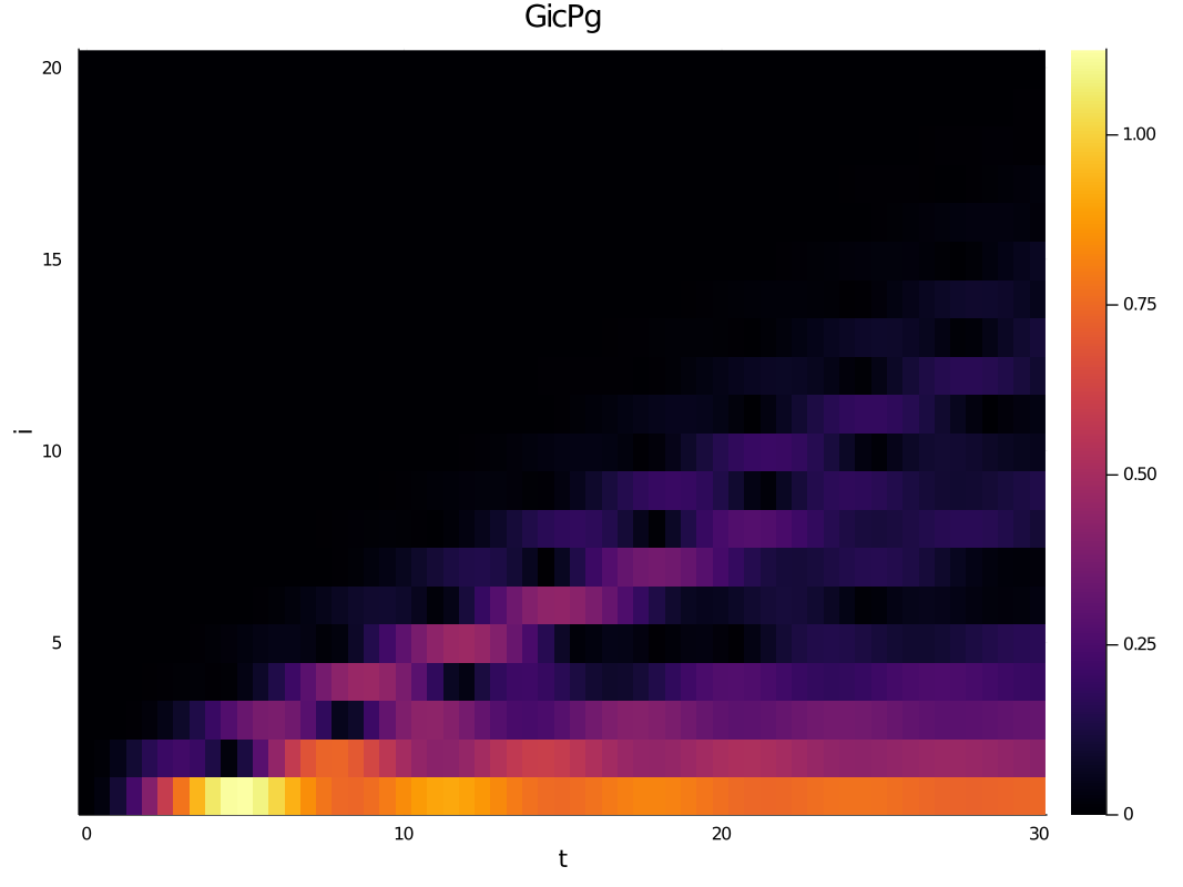
ob3 = TwoSiteObservable("SXdisp", sx, disp(d), [1], collect(2:N+1))

will measure $\langle\sigma_x\hat{q}_i\rangle$ where $\hat{q}_i$ is the displacement operator of the chain site and the index i runs over all chain sites.

Finally we launch the simulation with the function runsim.

dt = 0.5
T = 30.0

A, dat = runsim(dt, T, A, H;
                name = "ohmic spin boson model",
                method = :TDVP1,
                obs = [ob2,ob3],
                convobs = [ob1],
                params = @LogParams(N, d, α, Δ, ω0, s),
                convparams = [2,4,6],
                verbose = false,
                save = true,
                plot = true,
                );

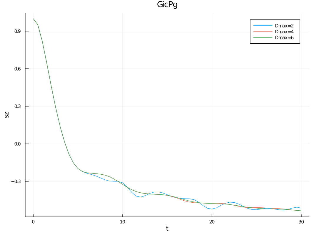
This will propagate the MPS up to time T in time steps of dt. The simulation will be performed using 1-site TDVP with bond-dimensions of 2, 4 and 6 in order to check for convergence. The observables supplied to convobs will be measured at every time step for every bond-dimension, while the observables supplied to obs will only be measured for the last (most accurate) convergence parameter supplied to convparams.

The final MPS is returned to A and the measurement data is returned to dat. If the option save=true is used the data will also be saved to a file. The directory in which data should be saved may be passed to the keyword argument savedir; by default the save directory is ~/MPSDynamics, which will be created if it doesn't exist (if using Windows the slashes will need to be reversed). The data directory name can be changed with the keyword argument unid.

If the option plot=true is used, plots for 1D observables will be automatically generated and saved along with the data.

Otherwise plots can be produced from dat, e.g.

using Plots
plot(dat["data/times"], dat["convdata/sz"],label=["Dmax=2" "Dmax=4" "Dmax=6"], xlabel="t",ylabel="sz", title="")
heatmap(dat["data/times"], collect(1:N), abs.(dat["data/SXdisp"][1,:,:]), xlabel="t",ylabel="i", title="")

The data is stored in the JLD format which is based on HDF5. Loading the data in Julia using the JLD package will recover the full type information of the Julia variables that were stored. At the same time the HDF5 format is natively supported across many platforms and languages. For example, to load the spin-z data in Mathematica one could do

Import["~/MPSDynamics/XXXXX/dat_XXXXX.jld",{"HDF5","Datasets","/data/sz"}]

Documentation

https://shareloqs.github.io/MPSDynamics/

Publications

Publications which make use of MPSDynamics:

• Lacroix et al. From Non-Markovian Dissipation to Spatiotemporal Control of Quantum Nanodevices. Quantum 8, 1305, April 2024

  • https://doi.org/10.22331/q-2024-04-03-1305

• Riva et al. Thermal cycle and polaron formation in structured bosonic environments. Phys. Rev. B 108(19):195138, November 2023

  • https://doi.org/10.1103/PhysRevB.108.195138

• Lacroix et al. Unveiling non-Markovian spacetime signaling in open quantum systems with long-range tensor network dynamics. Phys. Rev. A 104(5):052204, November 2021

  • https://link.aps.org/doi/10.1103/PhysRevA.104.052204

• Dunnett et al. Influence of non-adiabatic effects on linear absorption spectra in the condensed phase: Methylene blue. J. Chem. Phys. 155(14):144112, October 2021

  • http://aip.scitation.org/doi/10.1063/5.0062950

• Dunnett and Chin. Simulating quantum vibronic dynamics at finite temperatures with many body wave functions at 0K. Front. Chem. 8, January 2021

  • https://doi.org/10.3389/fchem.2020.600731

• Dunnett and Chin. Matrix Product State Simulations of Non-Equilibrium Steady States and Transient Heat Flows in the Two-Bath Spin-Boson Model at Finite Temperatures. Entropy 23(1), January 2021

  • https://doi.org/10.3390/e23010077

Data Repositories

• Exact Spin-Boson-Model Tunneling Dynamics with Time Dependent Variation Matrix Product States (TDVMPS). Barrier height and temperature parameter space.

  • 10.5281/zenodo.4432014

• Real-time benchmark dynamics of the Ohmic Spin-Boson Model computed with Time-Dependent Variational Matrix Product States. (TDVMPS) coupling strength and temperature parameter space.

  • 10.5281/zenodo.4352728

Citation

If you use this package in your research, please cite it:

• Dunnett, A. (2021). angusdunnett/MPSDynamics: (v1.0). Zenodo. https://doi.org/10.5281/zenodo.5106435

How to Contribute

Contributions are welcome! Don't hesitate to contact us if you

• found a bug;
• have a suggestion on how to improve the code and/or documentation;
• would like to get involved in writing code and/or documentation.

References

Footnotes

1. D. Tamascelli, A. Smirne, J. Lim, S. F. Huegla, and M. B. Plenio, Physical Review Letters 123, 090402 (2019) arXiv: 1811.12418 ↩

2. J. Haegeman, C. Lubich, I. Oseledets, B. Vandereycken, and F. Verstraete, Physical Review B 94, 165116 (2016), arXiv: 1408.5056 ↩ ↩²

3. A. J. Dunnett & A. W. Chin, Physical Review B, 104(21), 214302 (2021) ↩