ABM

Agent based model framework to simulate collective foraging with visual private and social cues

Running the Application

This repository hold the code base for the agent based model framework implemented in python/pygame to model and simualate agents collectively foraging in the environment.

(No GUI) Runnning with docker or docker-compose

The application is fully dockerized (only in headless/no gui mode) so that your only requirement is a docker/docker-compose compatible system, with installed docker and docker-compose.

docker-compose

Then simply navigate to the repo, initialize the experiment you would like to carry out in abm/data/metaprotocol/experiments/docker_exp.py then run the simulation in headless mode with docker-compose up. The saved data will appear in the abm/data/simulation_data. After running the container remove it with the attached volumes with docker-compose down -v. You can decide if you want to build the image locally or use the latest stable (refelcting state on develop) image from DockerHub. To switch between these follow the instructions (in comment) in the docker-compose.yml file.

docker

If docker-compose is not available you can use the following pure docker commands instead: Be sure, that you are in the root ABM folder (in which e.g. .env file is present) then (pull and) run the application as follows:

docker run -it --mount type=bind,source="/$(pwd)/abm/data",target=/app/abm/data --name scioip34abmcontainer mezdahun/scioip34abm:latest

In case the image has not yet been pulled on your system (from DockerHub) it will be now. Then the host machine's abm/data folder will be bind-mounted to the container's corresponding folder so that the experiment to be run can be changed from the host, and the generated data will be visible on the host.

After running the container don't forget to cleanup. Remove the container and the image (if you don't want to use it anymore):

docker rm scioip34abmcontainer -v
docker rmi mezdahun/scioip34abm:latest

(With GUI) Running without docker

In case you would like to interact with the filesystem or the application (with GUI) while runnning it, first install it's requirements and run the application as follows

Requirements

To run the simulations you will need python 3.8 or 3.9 and pip correspondingly. It is worth to set up a virtualenvironment using pipenv or venv for the project so that your global workspace is not polluted.

Test Requirements

To test if all the requirements are ready to use:

1. Clone the repo
2. Activate your virtual environment (pipenv, venv) if you are using one
3. Move into the cloned repo where setup.py is located and run pip install -e . with that you installed the simulation package
4. run the start entrypoint of the simulation package by running playground-start or abm-start
5. If you also would like to save data you will need an InfluxDB instance. To setup one, please follow the instructions below.
6. If you would like to run simulations in headless mode (without graphics) you will need to install xvfb first (only tested on Ubuntu) with sudo apt-get install xvfb. After this, you can start the simulation in headless mode by calling the headless-abm-start entrypoint instead of the normal abm-start entrypoint.

Install Grafana and InfluxDB

To monitor individual agents real time and save simulation data (i.e. write simulation data real time and save upon request at the end) we use InfluxDB and a grafana server for visualization. For this purpose you will need to install influx and grafana. If you don't do these steps you are still going to be able to run simulations, but you won't be able to save the resulting data or visualize the agent's parameters. This installation guide is only tested on Ubuntu. If you decide to use another op.system or you don't want to monitor and save simulation data, set USE_IFDB_LOGGING and SAVE_CSV_FILES parameters in the .env file to 0.

Click to expand for Grafana and InfluxDB installation details!

Install Grafana

1. run the following commands to add the grafana APT repository and install grafana

wget -q -O - https://packages.grafana.com/gpg.key | sudo apt-key add -
echo "deb https://packages.grafana.com/oss/deb stable main" | sudo tee -a /etc/apt/sources.list.d/grafana.list
sudo apt-get update
sudo apt-get install -y grafana

2. enable and start the grafana server

sudo /bin/systemctl enable grafana-server
sudo /bin/systemctl start grafana-server

3. as we will use real time monitoring we have to change the minimal graph refresh rate in the config file of grafana.

   1. use sudo nano /etc/grafana/grafana.ini to edit the config file
   2. use Ctrl + W to serach for the term min_refresh_interval
   3. change the value from 5s to 100ms
   4. delete the commenting ; character from the beginning of the row
   5. save the file

4. restart your computer with sudo reboot

5. you can now check your installation. Open a browser on the client PC and go to http://localhost:3000. You’re greeted with the Grafana login page.

6. Log in to Grafana with the default username admin, and the default password admin.

7. Change the password for the admin user when asked.

Install influxdb:

1. Use the following commands to add InfluxDB APT repository and install InfluxDB

wget -qO- https://repos.influxdata.com/influxdb.key | sudo apt-key add -
source /etc/os-release
echo "deb https://repos.influxdata.com/debian $(lsb_release -cs) stable" | sudo tee /etc/apt/sources.list.d/influxdb.list
sudo apt update && sudo apt install -y influxdb

2. Start and enable the service

sudo systemctl unmask influxdb.service
sudo systemctl start influxdb
sudo systemctl enable influxdb.service

3. Use the following commands to initialize a home InfluxDB instance and grant priviliges to grafana. Please note that in general passwords should not be uploaded to github. We are doing it now as this process is not sensitive (saving simulation data on local database) and doesn't make sense to parametrize the password.

influx --execute "create database home"
influx --execute "use home"
influx --execute "create user monitoring with password 'password' with all privileges"
influx --execute "grant all privileges on home to monitoring"
influx --execute "show users"

4. after the last command you will see this

user admin

---

grafana true

Connect Grafana with Influx

(the following instructions were copied from Step4. of this source)

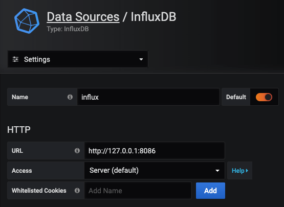
Now we have both Influx and Grafana running, we can stitch them together. Log in to your Grafana instance and head to “Data Sources”. Select “Add new Data Source” and find InfluxDB under “Timeseries Databases”.

As we are running both services on the same Pi, set the URL to localhost and use the default influx port of 8086:

Image

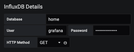
We then need to add the database (home), user (monitoring) and password (password) that we set earlier:

Image

That’s all we need! Now go ahead and hit “Save & Test” to connect everything together. You will see a "Data source is working" message

Import Dashboard from repo

1. Open your grafana app from the browser and on the left menu bar click on the "+" button and the on the "Import button"
2. Upload the json file (that holds the blueprint of the grafana dashboard) from the repo under the path abm/data/grafana_dashboard.json

(HPC) Using singularity on HPC

To run experiments on cluster nodes of the HPC we need to use singularity, as docker is not directly allowed on cluster nodes. To do so, first we need to transform the automatically built docker image on DockerHub to an immutable singularity image (SIF file). This can be done on any linux based host computer with sudo privileges and installed singularity (v3.7.0).

Choose a local host machine with sudo right.

1. Install singularity on host with this or this method.
2. Pull and build docker image to sif file: sudo singularity build scioip34abm.sif docker://mezdahun/scioip34abm. Note that the container always represents the develop branch and only rebuilt when another branch is merged or a push event is carried out on develop.
3. Use sshfs to create a mount between your linux system and the HPC gateway
4. Then upload your sif image into the mount (copy)

After this point you will have a SIF file on the home folder of your user gateway and from this point you will work on the gateway.

5. Now you have to clone the codebase (this repo) to the home directory of user gateway.
6. Copy the SIF file from the home folder of the gateway into this new cloned ABM folder and cd into it.
7. As we will bind the data codebase to the singularity containers (so that we can dynamically define new experiments without rebuilding the base image) we can now prepare these experiments as experiment <eperiment name>.py files under abm/data/metaprotocol/experiments. Corresponding .env files will be generated automatically later on. Only keep those experiment files in this folder that you will run on the cluster. Move all other experiment files into the archive subfolder. As again, we will run ALL of the experiment files in abm/data/metaprotocol/experiments keep only those there that you want to run to avoid cluttering the cluster with unwanted jobs.
8. After this point you can call the bash script HPC_run_all_exp.sh as sh HPC_run_all_exp.sh. This will take care of initializing the folder structure, mounting volumes to the individual singularity containers on the nodes and running the experiments in individual singularity instances based on the SIF image you created.
9. ALL the data will be generated under abm/data/simulation_data as it would be expected with local runs of experiments due to beegfs connection between the gateway and the nodes.
10. These you can use on any host by mounting your gateway to the host with sshfs
11. Log messages and error messages will be saved into a new slurm_log folder in the ABM folder

Heavily distributed runs on cluster nodes

In the HPC_run_all_exp.sh bash script we use the sbatch flag --exclusive to avoid any other jobs running on the given node. This is a wasteful behavior but it separates individual instances of the simulation maximally. To use multiple simulation instances on the same node use the HPC_run_all_exp_distributed.sh script. When run in a distributed way 4CPU will be dedicated per instance on the cluster nodes and no other user can use the node at the same time (but other jobs of the same user can). Saving data happens in the same shared influxdb instance (per node). The final data folder structure is different than in previous cases. To distrivute a given experiment.py file on many instances and nodes we first copy this file into N copies each of which is hashed with a random string (as well as the corresponding env files are generated). The number of instances can be controlled with the environment variable NUM_INSTANCES_PER_EXP when calling the bash script. Each resulting singularity instance will generate K batches (this should be set to 1 in the experiment files for maximal usage of parallel computing). At the end in the simulation_data folder you will see multiple hashed subfolders starting with the name of the original experiment. Each of these are generated parallely on different instances and nodes. You can merge these into the old folder structure (so that it can be replayed or summarized later on with data processing tools) with the abm/data/metaprotocol/experiments/archive/organize_distributed_experiment.py script. To do so, first copy all hashed folders into a subfolder with the name of the experiment. Then change the path in the script to this folder and run the script. This will create the adequate folder structure and delete hashed folders.

Example workflow

1. ssh into the gateway (after preparing the codebase and the SIF image as decribed before)
2. pull the repo and prepare your experiment file under abm/data/metaprotocol/experiments and move all other (unused) files from this folder to the archive subfolder
3. when preparing your experiment use the following parameters to declare your MetaRunner instance.

EXP_NAME = os.getenv("EXPERIMENT_NAME", "")
if EXP_NAME == "":
    raise Exception("No experiment name has been passed")
    
description_text = "Lorem Ipsum..."
    
mp = MetaProtocol(experiment_name=EXP_NAME, num_batches=1, parallel=True,
                  description=description_text, headless=True)

It is important that you:

• Pass the experiment name from the environment when running distributed from the HPC
• You only use single batch (num_batches=1) experiments. Multiple batches will be defined via sbatch automatically.
• Set your experiment to parallel (so that multiple instances can use the same InfluxDB instance) and headless (so that no visualization will be used)

4. Run your experiment in a distributed way on N individual instances on the HPC with

NUM_INSTANCES_PER_EXP=<N> sh HPC_run_all_exp_distributed.sh

5. N hashed (with random string) .envfile will appear as well as your experiment file will be copied N times.
6. You can check your running instances with squeue -u <your username>
7. You can find the log files under the slurm_logs folder and you can continously read the logs of a given slurm job with watch tail -n 30 slurm_logs/.<job id>.log. Error files are generated in the same way but with .err extension
8. After the instances are done copy all hashed folders into a common folder. Then change the path in the abm/data/metaprotocol/experiments/archive/organize_distributed_experiment.py to this common folder and run the script.
9. You end up having 1 folder (in which you copied the hashed subfolders originally) but instead of the hashed subfolder structure you will have N batch folders with the name batch_<i>

Details of the package

In this section the package is detailed for reproducibility and for ease of use. Among others you can read about the main restrictions and assumptions we used in our framework, how one can initialize the package with different parameters through .env files, and how the code is structured.

4. run your experiment file

Code Elements

The code is structured into a single installable python package called abm. Submodules of this package contain the main classes and methods that are used to implement the functionalities of our framework, such as Agent, Resource and Simulation classes among others. A dedicated contrib submodule provides parameters for running the simulations in python syntax. These parameters are either initialized from a .env file (described later) or they are not to be changed throughout simulations (such as passwords and database details) and therefore fixed in these scripts. Note that although we store passwords as text these are absolutely insensitive as they are only needed locally on a simulation computer to access the database in which we store simulation data (that is by nature not sensitive data).

Submodules

The package includes the following submodules:

• agent: including the Agent class implementing a simple interactive agent that is able to move in the environment, update it's appearence in pygame, use visual social cues, find resource patches and exploit them. All necessary method that implements these behaviors are packed in the class and called in the update method that is used to update the agents status (position, orientation, exploited resources, decision parameters) in each timestep by pygame. This class inherits from the pygame.Sprite class and therefore can be used accordingly. A helper script of the submodule supcalc.py inlcudes some independent functions to calculate distances, norms, angles, etc.
• contrib: including helper parameters of the package that can be later imported as abm.contrib.<name_of_param_bundle>. For further information about what the individual parameter bundles include within this submodule please read the comment in the beginning of these scripts.
• environment: including classes and methods for environmental elements. As an example it includes the Resource class that implements a resource patch in the environment. Similar to the Agent class it inherits from pygame sprites and therefore the update method will call all relevant methods in each timestep.
• loader: including all classes and methods to dynamically load data that was generated with the package. These methods are for example cvs and json readers and initializers that initialize input classes for Replay and DataAnalysis tools.
• metarunner: including all classes and methods to run multiple simulations one after the other with programatically changed initialization parameters. The main classes are Tunables that define a criterion range with requested number of datapoints (e.g.: simulate with environment width from 300 to 600 via 4 datapoints). The Constant class that defines a fixed criterion throughout the simulations (e.g.: keep the simulation time T fixed at 1000). And MetaProtocol class that defines a batch of simulations with all combinations of the defined criteria according to the added Tunables and Constants. During running metaprotocols the corresponding initializations (as .env files) will be saved under the data/metaprotocol/temp folder. Only those .env files will be removed from here for which the simulations have been carried out, therefore the metaprotocol can be interrupted and finished later.
• monitoring: including all methods to interface with InfluxDB, Grafana and to save the stored data from the database at the end of the simulation. The data will be saved into the data/simualtion_data/<timestamp_of_simulation> of the root abm folder. The data will consist of 2 relevant csv files (agent_data, resource_data) containing time series of the agent and resource patch status and a json file containing all parameters of the simulation for reproducibility.
• simulation: including the main Simulation class that defines how the environment is visualized, what interactions the user can have with the pygame environment (e.g.: via cursor or buttons), and how the environment enforces some restrictions on agents, and how resources are regenerated. Furthermore a PlaygroundSimulation class is dedicated to provide an interactive playground where the user can explore different parameter combinations with the help of sliders and buttons. This class inherits all of it's simulation functionality from the main Simulation class but might change the visualization and adds additional interactive optionalities. When the framework is started as a playground, the parameters in the .env file don't matter anymore, but a .env file is still needed in the main ABM folder so that the supercalss can be initiated.
• replay: to explore large batches of simulated experimental data, a replay class has been implemented. To initialize the class one needs to pass the absolute path of an experiment folder generated by the metaruneer tool. Upon initialization, in case the experiment is not yet summarized into numpy arrays this step is carried out. The arrays are then read back to the memory at once. The different batches and parameter combinations can be explored with interactive GUI elements. In case the amount of data is too large, one can use undersampling of data to only include every n-th timestep in the summary arrays.

Functionality and Behavior

Here you can read about how the framework works in large scale behavior and what restrictions and assumptions we used throughout the simulation.

Behavior

Upon starting the simulation an arena will pop up with given number of agents and resource patches. Details of these are controlled via .env variables and you can read more below. Agents will search for hidden resource patches and exploit/consume these with a given rate (resource unit/time) when found. The remaining resource units are shown on the patches as well as their quality (how much unit can be exploited in a time unit per agent).

Agents can behave according to 3 distinct behavioral states. These are: Exploration (individual uninformed state looking for resources with random movement and integration of individual and social cues in the meanwhile). Relocation (informed state in which the agent "decides" to join to another agent's patch). Exploitation (in which the agent consumes a resource patch and is recognized as a social visual cue for other agents). The mode of the agents are depicted with their colors, that is blue, purple and green respectively. Agents can collide with each other (red color) and in this case they avoid the collision by turning away from the other agents. Collision can be turned off during exploitation (ghost mode). Recognizing exploiting agents as social cues on the same patch can be turned off.

Each social cue (other exploiting agent) creates a visual projection on the focal agent's retina if in visual range (and the limited FOV allows). Relocation happens according to the overall excitation of the agent's retina. The focal agent steers right if the right hemifield is more excited and left if the left hemifield is more excited.

During exploitation agents slow down and stop on patches.

Agents decide on which mode to enter via a dedicated decision process. The decision process continously integrates private information (Did I find a new patch? How good the quality of the new patch is?) and social information (Do I see any other agents axploiting nearby? How many/how close according to visual projection field?). With the parameters of the decision process one con control how socially susceptible agents are and how much being in e.g. relocation inhibits exploitation and vica versa. Agents integrate infromation all the time and they can deliberately stop being in a behavioral mode to switch into another.

Interaction

During the simulation visualization can be turned off to speed up the run. In case it is turned on, the user is able to interact with the simulation as follows:

• click (left) and move agents in space
• rotate agents with mouse scroll
• pause/unpause simulation with space
• show social visual field with return
• increase/decrease framrate with f/s
• reset default framerate with d

Environment variables as parameters

To parametrize the simulation we use .env files. These include the main parameters line by line. This means, that a single .env file defines a simulation run fully. The env variables are as follows:

Click to see all env variables!

• N: number of agents
• N_RESOURCES: number of resource patches
• T: number of simulation timesteps
• INIT_FRAMERATE: default framerate when visualization is on. Irrelevant for when visualization is turned off
• WITH_VISUALIZATION: turns visualization on or off
• VISUAL_FIELD_RESOLUTION: Resolution/size of agents' visual projection fields in pixels
• ENV_WIDTH: width of the environment in pixels
• ENV_HEIGHT: height of the environment in pixels
• RADIUS_AGENT: radius of agents in pixels
• RADIUS_RESOURCE: radius or resource patches in pixels
• MIN_RESOURCE_PER_PATCH: minimum contained resource units of a resourca patch. real value will be random uniform between min and max values.
• MAX_RESOURCE_PER_PATCH: maximum contained resource units of a resourca patch.
• REGENERATE_PATCHES: turns on or off resource patch regeneration upon full depletion.
• AGENT_CONSUMPTION: maximum resource consumption of agents (per time unit). Can be lower according to resource patch quality
• MIN_RESOURCE_QUALITY: minimum quality of resourca patch. real quality will be random uniform between min and max quality.
• MAX_RESOURCE_QUALITY: maximum quality of resource patches.
• TELEPORT_TO_MIDDLE: pulling exploiting agents into the middle of the resource patch if turned on.
• GHOST_WHILE_EXPLOIT: disabling collisions when the agents exploit when turned on.
• PATCHWISE_SOCIAL_EXCLUSION: not taking into consideration agents on the same patch as social cues if turned on.
• AGENT_FOV: Field of view of the agents. FOV is symmetric and defined with percent of pi. e.g if 0.6 then fov is (-0.6pi, 0.6pi). 1 is full 360 degree vision
• VISION_RANGE: visual range in pixels
• VISUAL_EXCLUSION: taking visual exclusion into account when calculating visual cues if turned on.
• SHOW_VISUAL_FIELDS: always show visual fields of agents when turned on.
• SHOW_VISUAL_FIELDS_RETURN: show visual fields of agents when return pressed if turned on
• SHOW_VISION_RANGE: visualizing visual range and field of view of agents when turned on.
• USE_IFDB_LOGGING: logs simulation data into a connected InfluxDB database when turned on (and InfluxDB is initialized)
• SAVE_CSV_FILES: saves data from connected InfluxDB instance as csv files if turned on.

Parameters of the decision process as decsribed in rpopsal:

• DEC_TW: time constant of w process
• DEC_EPSW: social excitability
• DEC_GW: social decay
• DEC_BW: social process baseline
• DEC_WMAX: social process limit
• DEC_TU: time constant of u process
• DEC_EPSU: individual excitability
• DEC_GU: individual decay
• DEC_BU: individual process baseline
• DEC_UMAX: individual process limit
• DEC_SWU: social to individual inhibition
• DEC_SUW: individual to social inhibition
• DEC_TAU: novelty time window of private information
• DEC_FN: novelty multiplier
• DEC_FR: quality multiplier

Movement parameters:

• MOV_EXP_VEL_MIN: minimum exploration velocity
• MOV_EXP_VEL_MAX: maximum exploration velocity
• MOV_EXP_TH_MIN: minimum exploration orientation change (per time unit)
• MOV_EXP_TH_MAX: maximum exploration orientation change (per time unit)
• MOV_REL_DES_VEL: relocation velocity
• MOV_REL_TH_MAX: relocation maximal orientation change
• CONS_STOP_RATIO: deceleration during exploitation

Running multiple simulations at the same time

Metarunner API

To carry out multiple simulations fast (without visualizations), exploring parameter ranges in a clean and programatic way, a dedicated API has been created called metarunner. On can define parameter ranges (and desired values by first creating so called simulation "critera" as Tunable and Constant calss instances with parameter names and values. To know what parameters to fix and tune see parameter descriptions in the previous block. Once criteria has been defined, one can create a MetaProtocol instance and add the defined criteria. After this, the MetaProtocol instance can be run, meaning all defined parameter combinations will be used to carry out simulations. The resulting data will be generated under data/simulation_data/<experiment_name>/batch_<batch_id>/<simulation_timestamp>. Experiment files are dedicated python files (.py) using the metarunner API of the package to define and easily run such MetaProtocol instances. All runs during running a MetaProtocol are initialized with the help of .env files. An example of such an experiment file can be found in data/metaprotocol/experiments/exp1.py that can be simply run as:

python path_to_exp_file.py

Note that an initial .env file must exist under the root ABM folder.

Connected Tunables

It can happen that during an experiment one would like to change parameters together, e.g. such that they keep their product as a fixed number. For example, one might want that the total number of resources (number of patches X unit per patch) soulf remain the same for all runs and batches. To fix the product of parameters one can define TunedPairRestrain criterion, initializing with parameter1, parameter2 and product. During initialization of the metarunner all env files where this criterion does not hold will be deleted. If the relationship is quadratic, i.e. we want param1 x param2 ** 2 to be fixed as product we can use the add_quadratic_tuned_pair method instead of the add_tuned_pair method of the MetaProtocol class. You can see an example in the experiment file exp8.py.

Parallel Run of MetaProtocols

To carry out simulations parallel to each other (so that we can increase simulation speed) one needs to pay attention how the simulations (defined in experiment files) are started. In case we run multiple MetaProtocol instances at the same time, we have to set the attribute parallel of the MetaProtocol class instance to True, as well as we must define an experiment name (experiment_name attribute of MetaProtocol class). Furthermore, as now we need to initialize different metaprotocol classes with different .env files we also need to define how this happens. To do so here is a general recipe:

• create as many copies of an initial .env file in the root ABM directory as many parallely running MetaProtocol instances will be present. This is outside of the package ABM/abm directory.
• name these .env files as exp1.env, exp2.env, ..., expN.env
• open as many terminals as many parallely running MetaProtocol instances will be present.
• create as many experiment files as many parallely running MetaProtocol instances will be present.
• name these experiment files as exp1.py, exp2.py, ..., expN.py
• in each experiment file the criteria are defined and added to a MetaProtocol instance that has parallel set to True and has an experiment_name attribute.
• in each terminal i run the following command:

EXPERIMENT_NAME=exp<i> python <path_to_exp_file_folder>/exp<i>.py

Note that the parantheses denote variable indices and paths according to where you store your experiment files and which terminal you are at. A concrete example could be:

EXPERIMENT_NAME=exp4 python home/ABM/abm/data/metarunner/experiments/exp4.py

where we assume you have a exp4.env file in the root project folder (home/ABM) and you store an experiment file exp4.py under a dedicated path, in the example, this path is home/ABM/abm/data/metarunner/experiments/.

Note that the env variable EXPERIMENT_NAME is used to show the given MetaProtocol instance which .env file it needs to use (and replace during runs). Therefore it must have a scope ONLY for the given command. If you set this varaible globally on your OS then all MetaProtocol instances will try to use and replace the same .env file and therefore during parallel runs unwanted behavior and corrupted data states can occur. The given commands are only to be used on Linux.

Interactive Exploration Tool

To allow users quick-and-dirty experimentation with the model framework, an interactive playground tool has been implemented. This can be started with playground-start after preparing the environment as described above.

Once the playground tool has been started a window will pop up with a simulation arena on the upper right part with a given number of agnets and resources. Parameters are initialized according to the contrib package. These parameters can be tuned with interactive sliders on the right side of the window. To get some insights of these parameters see the env variable descriptions above or click and hold the ? buttons next to the sliders.

Resource number and radius

When changing the number of resource patches and their radii, the tool automatically adjusts these to each other so that the total covered area in the arena will not exceed 30% of the arena surface. This is necessary as resources are initialized in a way that no overlap is present.

Fixed Overall Resource Units

When starting the tool the overall amount of resource units (summed over all patches of the arena) is fixed and can be controlled with the SUM_R slider. Changing this value will redistribute the amount of units between the patches in a way that the ratio of units in between tha patches will not change, and the depletion level of the patches also stays the same. In case this feature is turned off with the corresponding action button below the simulation arena, increasing the number of resource patches will increase the overall number of resources in the environment.

Detailed Information

To get more detailed information about resource patches and agents, click and hold them with the left mouse button. Note that this alos moves the agents. Other interactions such as rotating agents, pausing the simulation, etc. are the same as in the original simulation class. In case you would like to get an insight about all agents and resources use the corresponding action button under the simulation area. Note that this can slow down the simulation significantly due to the amount of text to be rendered on the screen.

Video Recording

To show the effect of parameter combinations and make experiments reproducable, you can also record a short video of particularly interesting phenomena. To do so, use the Record Video action button under the simulation arena. When the recording is started, the button turns red as well as a red "Rec" dot will pop up in the upper left corner. When you stop the recording with the same action button, the tool will save and compress the resulting video and save in the data folder of the package. Please note that this might take a few minutes for longer videos.

Other Function Buttons

Some boolean parameters can be turned on and off with the help of additional function buttons (below the visualization area). These are

• Turn on Ghost Mode: overalpping on the patches are allowed
• Turn on IFDB logging: in case a visualization through the grafana interface is required one can start IFDB logging with this button. By default it is turned off so that we can avoid a database writing overhead and the tool can be aslo started without IFDB installed on the system.
• Turn on Visual Occlusion: in case it is turned on, agents can occlude visual cues from farther away agants.

Replay Tool

To visualize large batches of data generated as experiment folders with the metarunner tool, one can use the replay tool. A demonstrative script has been provided in the repo to show how one can start such a replay of experiment.

Behavior

Upon start if the experiment was not summarized before into numpy arrays this will be done. Then these arrays are read back to the memory to initialize the GUI of the tool. On the left side an arena shows the agnets and resources. Below, global statistics are shown in case it is requested with the Show Stats action button. The path of the agents as well as their visual field can be visualized with the corresponding buttons. Note that interactions from the simulation or the playground tool won't work here as this visualization will be a pure replay (as in a replayed video) of the recorded simulation itself. One can replay the recorded data in time with the Start/Stop button or by moving the time slider.

Parameter Combinations

Possible parameter combinations are read automatically from the data and the corresponding sliders will be initialized in the action area accordingly. By that, one can go through the simulated parameter combinations and different batches by moving the sliders on the right.

Plotting

To plot some global statistics of the data corresponding action buttons have been implemented on the right. Note that it only works with 1, 2 or 3 changed parameters. In case 3 parameters were tuned throughout the experiment one can either plot multiple 2 dimensional figures or "collapse" the plot along an axis using some method, such as minimum or maximum collision. This means that along that axis instead of taking all values into consideration one will onmly take the max or min of the values. This is especially useful when 2 parameters were tuned together in a way that their product should remain the same (That can be done adding so called Tuned Pairs to the criterion of the metarunner tool). In these cases only specified parameter combinations have informative values and not the whole parameter space provided with the parameter ranges.