
ReLife is an open source Python library for asset management based on reliability theory and lifetime data analysis.
- Survival analysis: non-parametric estimator (Kaplan-Meier), parametric estimator (Maximum Likelihood) and regression models (Accelerated Failure Time and Parametric Proportional Hazards) on left-truncated, right-censored and left-censored lifetime data.
- Reliability theory: optimal age of replacement for time-based mainteance policy for one-cycle or infinite number of cycles, with exponential discounting.
- Renewal theory: expected number of events, expected total costs or expected number of replacements for run-to-failures or age replacement policies.
From PyPI:
pip3 install relifeThe official documentation is available at https://rte-france.github.io/relife/.
@misc{relife,
    author = {T. Guillon},
    title = {ReLife: a Python package for asset management based on
    reliability theory and lifetime data analysis.},
    year = {2022},
    journal = {GitHub},
    howpublished = {\url{https://github.com/rte-france/relife}},
}Icon made by Freepik from Flaticon.
The following example shows the steps to develop a preventive maintenance policy by age on circuit breakers:
- Perform a survival analysis on lifetime data,
- Compute the optimal age of replacement,
- Compute the expected total discounting costs and number of expected replacements for the next years.
The survival analysis is perfomed by computing the Kaplan-Meier estimator and fitting the parameters of a Weibull and a Gompertz distribution with the maximum likelihood estimator.
import numpy as np
import matplotlib.pyplot as plt
from relife.datasets import load_circuit_breaker
from relife import KaplanMeier, Weibull, Gompertz, AgeReplacementPolicy

time, event, entry = load_circuit_breaker().astuple()
km = KaplanMeier().fit(time,event,entry)
weibull = Weibull().fit(time,event,entry)
gompertz = Gompertz().fit(time,event,entry)
The results of fitting the Weibull and Gompertz distributions are compared by looking at the attributes weibull.result.AIC and gompertz.result.AIC. The Gompertz distribution gives the best fit and will be chosen for the next step of the study. The code below plots the survival function obtained by the Kaplan-Meier estimator and the maximum likelihood estimator for the Weibull and Gompertz distributions.
km.plot()
weibull.plot()
gompertz.plot()
plt.xlabel('Age [year]')
plt.ylabel('Survival probability')
We consider 3 circuit breakers with the following parameters:
- the current ages of the circuit breakers are a0 = [15, 20, 25] years,
- the preventive costs of replacement are evaluated cp = 10 k€,
- the failure costs (e.g. lost energy) are evaluated cf = [900, 500, 100] k€,
- the discount rate is rate = 0.04.
a0 = np.array([15, 20, 25]).reshape(-1,1)
cp = 10
cf = np.array([900, 500, 100]).reshape(-1,1)
policy = AgeReplacementPolicy(gompertz, a0=a0, cf=cf, cp=cp, rate=0.04)
policy.fit()
policy.ar1, policy.ar
Where ar1 are the time left until the first replacement, whereas ar is the optimal age of replacement for the next replacements:
(array([[10.06828465],
        [11.5204334 ],
        [22.58652687]]),
 array([[20.91858994],
        [25.54939328],
        [41.60855399]]))
The optimal age of replacement minimizes the asymptotic expected equivalent annual cost. It represents the best compromise between replacement costs and the cost of the consequences of failure.
a = np.arange(1,100,0.1)
za = policy.asymptotic_expected_equivalent_annual_cost(a)
za_opt = policy.asymptotic_expected_equivalent_annual_cost()
plt.plot(a, za.T)
for i, ar in enumerate(policy.ar):
    plt.scatter(ar, za_opt[i], c=f'C{i}',
        label=f" cf={cf[i,0]} k€, ar={ar[0]:0.1f} years")
plt.xlabel('Age of preventive replacement [years]')
plt.ylabel('Asymptotic expected equivalent annual cost [k€]')
plt.legend()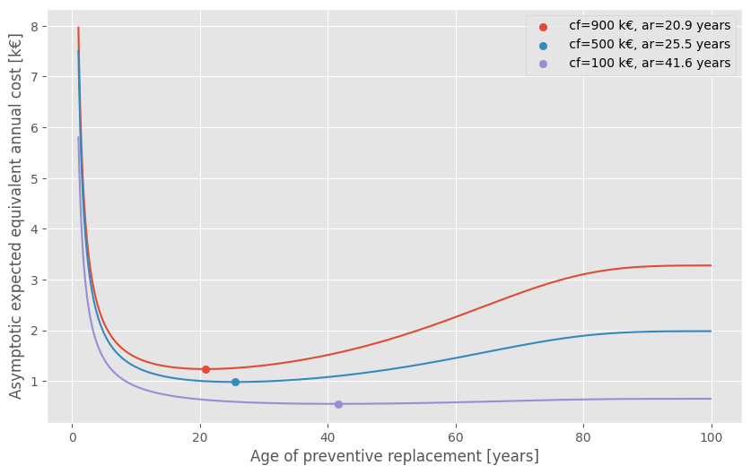
For budgeting, the expected total discounted costs for the 3 circuit breakers are computed and we can plot the total annual discounted costs for the next 30 years, including costs of failures and costs of preventive replacements.
dt = 0.5
step = int(1/dt)
t = np.arange(0, 30+dt, dt)
z = policy.expected_total_cost(t).sum(axis=0)
y = t[::step][1:]
q = np.diff(z[::step])
plt.bar(2020+y, q, align='edge', width=-0.8, alpha=0.8, color='C2')
plt.xlabel('Year')
plt.ylabel('Expected discounted annual cost in k€')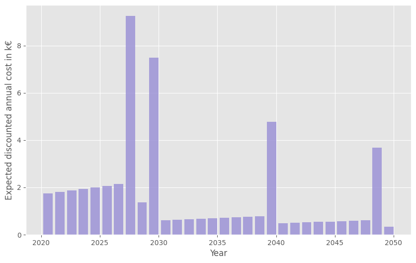
Then the total number of replacements are projected for the next 30 years. Failure replacements are counted separately in order to prevent and prepare the workload of the maintenance teams.
mt = policy.expected_total_cost(t, cf=1, cp=1, rate=0).sum(axis=0)
mf = policy.expected_total_cost(t, cf=1, cp=0, rate=0).sum(axis=0)
qt = np.diff(mt[::step])
qf = np.diff(mf[::step])
plt.bar(y+2020, qt, align='edge', width=-0.8, alpha=0.8,
    color='C1', label='all replacements')
plt.bar(y+2020, qf, align='edge', width=-0.8, alpha=0.8,
    color='C0', label='failure replacements only')
plt.xlabel('Years')
plt.ylabel('Expected number of annual replacements')
plt.legend()
The figure shows the expected replacements for the very small sample of 3 circuit breakers. When the population of assets is large, the expected failure replacements is a useful information to build up a stock of materials.
