Classification of default of credit card clients from the UCI dataset using machine learning techniques.
- Introduction
- Exploratory Data Analysis
- Data Preprocessing
- Classification algorithms
- Results
- Conclusions
The aim of this study is to exploit some supervised machine learning algorithms to identify the key drivers that determine the likelihood of credit card default, underlining the mathematical aspects behind the methods used. Credit card default happens when you have become severely delinquent on your credit card payments. In order to increase market share, card-issuing banks in Taiwan over-issued cash and credit cards to unqualified applicants. At the same time, most cardholders, irrespective of their repayment ability, the overused credit card for consumption and accumulated heavy credit and debts
The goal is to build an automated model for both identifying the key factors, and predicting a credit card default based on the information about the client and historical transactions. The general concepts of the supervised machine learning paradigm are later reported, together with a detailed explanation of all techniques and algorithms used to build the models. In particular, Logistic Regression, Random Forest and Support Vector Machines algorithms have been applied.
The analysis has been fully conducted with Python language, exploiting several machine learning and statistical frameworks available such as scikit-learn, numpy, pandas, imblearn together with other data visualization libraries (matplotlib and seaborn).
Some code snippets have been reported for a better understanding of each step. Moreover, the full code implementation of this analysis is publicly available at github.com/robertofranceschi/default-credit-card-prediction.
The dataset used in this study is the Default of credit card clients from the UCI machine learning repository, available at the following link.
It consists of 30000 observations that represent distinct credit card clients. Each observation has 24 attributes that contain information on default payments, demographic factors, credit data, history of payment, and bill statements of credit card clients in Taiwan from April 2005 to September 2005.
The first group of variables contains information about the client personal information:
ID: ID of each client, categorical variableLIMIT_BAL: Amount of given credit in NT dollars (includes individual and family/supplementary credit)SEX: Gender, categorical variable (1=male, 2=female)EDUCATION: level of education, categorical variable (1=graduate school, 2=university, 3=high school, 4=others, 5=unknown, 6=unknown)MARRIAGE: Marital status, categorical variable (1=married, 2=single, 3=others)AGE: Age in years, numerical variable
The following attributes contains information about the delay of the past payment referred to a specific month:
PAY_0: Repayment status in September 2005 (-1=pay duly, 1=payment delay for one month, 2=payment delay for two months, … 8=payment delay for eight months, 9=payment delay for nine months and above)PAY_2: Repayment status in August 2005 (same scale as before)PAY_3: Repayment status in July 2005 (same scale as before)PAY_4: Repayment status in June 2005 (same scale as before)PAY_5: Repayment status in May 2005 (same scale as before)PAY_6: Repayment status in April 2005 (same scale as before)
Other variables instead consider the information related to the amount of bill statement (i.e. a monthly report that credit card companies issue to credit card holders in a specific month):
BILL_AMT1: Amount of bill statement in September, 2005 (NT dollar)BILL_AMT2: Amount of bill statement in August, 2005 (NT dollar)BILL_AMT3: Amount of bill statement in July, 2005 (NT dollar)BILL_AMT4: Amount of bill statement in June, 2005 (NT dollar)BILL_AMT5: Amount of bill statement in May, 2005 (NT dollar)BILL_AMT6: Amount of bill statement in April, 2005 (NT dollar)
The following variables instead consider the amount of previous payment in a specific month:
PAY_AMT1: Amount of previous payment in September, 2005 (NT dollar)PAY_AMT2: Amount of previous payment in August, 2005 (NT dollar)PAY_AMT3: Amount of previous payment in July, 2005 (NT dollar)PAY_AMT4: Amount of previous payment in June, 2005 (NT dollar)PAY_AMT5: Amount of previous payment in May, 2005 (NT dollar)PAY_AMT6: Amount of previous payment in April, 2005 (NT dollar)
The last variable is the one to be predicted:
default.payment.next.month: indicate whether the credit card holders are defaulters or non-defaulters (1=yes, 0=no)
The main aim of the data is to discriminate clients that are predicted to credit card default the next month, according to the default.payment.next.month column which is set to “0” for non-defaulters and “1” for defaulters. Thus, it is a binary classification problem on a relatively unbalanced dataset, as shown in the following figure.

Class distribution
As can be seen, a number of 6.636 out of 30.000 (or 22.1%) of clients will default next month (i.e. has category 1).
In order to get a first look at how data is presented, some observations of the dataset are shown in the table below. No missing feature is recorded for any of the 30.000 samples.
The data appears already encoded and cleaned. However, by better inspecting some samples and statistics there are some observations to point out.
# read input
data = pd.read_csv(INPUT_PATH)
data.head()| ID | LIMIT_BAL | SEX | EDUCATION | MARRIAGE | AGE | PAY_0 | PAY_2 | PAY_3 | PAY_4 | ... | BILL_AMT4 | BILL_AMT5 | BILL_AMT6 | PAY_AMT1 | PAY_AMT2 | PAY_AMT3 | PAY_AMT4 | PAY_AMT5 | PAY_AMT6 | default.payment.next.month | |
|---|---|---|---|---|---|---|---|---|---|---|---|---|---|---|---|---|---|---|---|---|---|
| 0 | 1 | 20000.0 | 2 | 2 | 1 | 24 | 2 | 2 | -1 | -1 | ... | 0.0 | 0.0 | 0.0 | 0.0 | 689.0 | 0.0 | 0.0 | 0.0 | 0.0 | 1 |
| 1 | 2 | 120000.0 | 2 | 2 | 2 | 26 | -1 | 2 | 0 | 0 | ... | 3272.0 | 3455.0 | 3261.0 | 0.0 | 1000.0 | 1000.0 | 1000.0 | 0.0 | 2000.0 | 1 |
| 2 | 3 | 90000.0 | 2 | 2 | 2 | 34 | 0 | 0 | 0 | 0 | ... | 14331.0 | 14948.0 | 15549.0 | 1518.0 | 1500.0 | 1000.0 | 1000.0 | 1000.0 | 5000.0 | 0 |
| 3 | 4 | 50000.0 | 2 | 2 | 1 | 37 | 0 | 0 | 0 | 0 | ... | 28314.0 | 28959.0 | 29547.0 | 2000.0 | 2019.0 | 1200.0 | 1100.0 | 1069.0 | 1000.0 | 0 |
| 4 | 5 | 50000.0 | 1 | 2 | 1 | 57 | -1 | 0 | -1 | 0 | ... | 20940.0 | 19146.0 | 19131.0 | 2000.0 | 36681.0 | 10000.0 | 9000.0 | 689.0 | 679.0 | 0 |
5 rows × 25 columns
# Summary Statistics
data.describe()| ID | LIMIT_BAL | SEX | EDUCATION | MARRIAGE | AGE | PAY_0 | PAY_2 | PAY_3 | PAY_4 | ... | BILL_AMT4 | BILL_AMT5 | BILL_AMT6 | PAY_AMT1 | PAY_AMT2 | PAY_AMT3 | PAY_AMT4 | PAY_AMT5 | PAY_AMT6 | default.payment.next.month | |
|---|---|---|---|---|---|---|---|---|---|---|---|---|---|---|---|---|---|---|---|---|---|
| count | 30000.00 | 30000.00 | 30000.00 | 30000.00 | 30000.00 | 30000.00 | 30000.00 | 30000.00 | 30000.00 | 30000.00 | ... | 30000.00 | 30000.00 | 30000.00 | 30000.00 | 3.00e+04 | 30000.00 | 30000.00 | 30000.00 | 30000.00 | 30000.00 |
| mean | 15000.50 | 167484.32 | 1.60 | 1.85 | 1.55 | 35.49 | -0.02 | -0.13 | -0.17 | -0.22 | ... | 43262.95 | 40311.40 | 38871.76 | 5663.58 | 5.92e+03 | 5225.68 | 4826.08 | 4799.39 | 5215.50 | 0.22 |
| std | 8660.40 | 129747.66 | 0.49 | 0.79 | 0.52 | 9.22 | 1.12 | 1.20 | 1.20 | 1.17 | ... | 64332.86 | 60797.16 | 59554.11 | 16563.28 | 2.30e+04 | 17606.96 | 15666.16 | 15278.31 | 17777.47 | 0.42 |
| min | 1.00 | 10000.00 | 1.00 | 0.00 | 0.00 | 21.00 | -2.00 | -2.00 | -2.00 | -2.00 | ... | -170000.00 | -81334.00 | -339603.00 | 0.00 | 0.00e+00 | 0.00 | 0.00 | 0.00 | 0.00 | 0.00 |
| 25% | 7500.75 | 50000.00 | 1.00 | 1.00 | 1.00 | 28.00 | -1.00 | -1.00 | -1.00 | -1.00 | ... | 2326.75 | 1763.00 | 1256.00 | 1000.00 | 8.33e+02 | 390.00 | 296.00 | 252.50 | 117.75 | 0.00 |
| 50% | 15000.50 | 140000.00 | 2.00 | 2.00 | 2.00 | 34.00 | 0.00 | 0.00 | 0.00 | 0.00 | ... | 19052.00 | 18104.50 | 17071.00 | 2100.00 | 2.01e+03 | 1800.00 | 1500.00 | 1500.00 | 1500.00 | 0.00 |
| 75% | 22500.25 | 240000.00 | 2.00 | 2.00 | 2.00 | 41.00 | 0.00 | 0.00 | 0.00 | 0.00 | ... | 54506.00 | 50190.50 | 49198.25 | 5006.00 | 5.00e+03 | 4505.00 | 4013.25 | 4031.50 | 4000.00 | 0.00 |
| max | 30000.00 | 1000000.00 | 2.00 | 6.00 | 3.00 | 79.00 | 8.00 | 8.00 | 8.00 | 8.00 | ... | 891586.00 | 927171.00 | 961664.00 | 873552.00 | 1.68e+06 | 896040.00 | 621000.00 | 426529.00 | 528666.00 | 1.00 |
8 rows × 25 columns
For example, the following criticities can be observed:
- the column name
PAY_0should be renamed inPAY_1; - about
EDUCATIONandMARRIAGEthere are some undocumented categories; - the columns
PAY_nhave a minimum in -2 (undocumented) and a maximum equal to 8. So, it is likely that these attributes need to be rescaled. ### 2.2 Data Cleaning
The presence of errors in the dataset can be addressed in two ways:
- deleting of the rows associated with an error (paying attention to the number of lines with respect to the total number of observations);
- with a correction of the wrong attribute.
In our case the first method is applied to the categorical variables, by safely removing the unknown categories (since the total number of anomalous values is 399):
- Regarding the attribute
EDUCATIONthere are three categories not listed in the description of the dataset provided by the UCI website that corresponds to 0, 5, and 6. - While for
MARRIAGEwe can notice the presence of category 0 that does not correspond to any categories previously described.
while the second approach is applied to the PAY_n features, correcting them by adding 1 to each attribute and grouping together the resulting values of '0' and '-1' (since 0 does not correspond to any value previously described).
data['MARRIAGE'].value_counts()Out [6]:
2 15964
1 13659
3 323
0 54
Name: MARRIAGE, dtype: int64
data['EDUCATION'].value_counts()Out [7]:
2 14030
1 10585
3 4917
5 280
4 123
6 51
0 14
Name: EDUCATION, dtype: int64
# Payment delay description
data[['PAY_1', 'PAY_2', 'PAY_3', 'PAY_4', 'PAY_5', 'PAY_6']].describe()| PAY_1 | PAY_2 | PAY_3 | PAY_4 | PAY_5 | PAY_6 | |
|---|---|---|---|---|---|---|
| count | 29601.00 | 29601.00 | 29601.00 | 29601.00 | 29601.00 | 29601.00 |
| mean | -0.01 | -0.13 | -0.16 | -0.22 | -0.26 | -0.29 |
| std | 1.12 | 1.20 | 1.20 | 1.17 | 1.14 | 1.15 |
| min | -2.00 | -2.00 | -2.00 | -2.00 | -2.00 | -2.00 |
| 25% | -1.00 | -1.00 | -1.00 | -1.00 | -1.00 | -1.00 |
| 50% | 0.00 | 0.00 | 0.00 | 0.00 | 0.00 | 0.00 |
| 75% | 0.00 | 0.00 | 0.00 | 0.00 | 0.00 | 0.00 |
| max | 8.00 | 8.00 | 8.00 | 8.00 | 8.00 | 8.00 |
# Amount of given credit in NT dollars
data.LIMIT_BAL.describe()
Out[20]:
count 29601.00
mean 167550.54
std 129944.02
min 10000.00
25% 50000.00
50% 140000.00
75% 240000.00
max 1000000.00
Name: LIMIT_BAL, dtype: float64
The very high value of standard deviation has been further investigated. As can be seen, most of defaults are for credit limits 0-100,000 (and density for this interval is larger for defaults than for non-defaults).

Density plot of amount of given credit (LIMIT_BAL)
Another relevant point which could affect the classification performances is the correlation among features: the presence of strongly correlated features may lead to a decline in the performances of some classification algorithms which assume that the predictors are all independent. Another benefit from spotting correlation among features is that the same information may be encoded with less attributes, and this could lead to simpler final models. Indeed, some methods suffer from high dimensional datasets (especially distance based ones with a few number of samples), so reducing the dimensions of the feature vectors can make it more trustable and stable, if the discarded dimensions don’t affect significantly the total original information.
The Pearson’s correlation coefficient is a statistic that measures the linear correlation between a pair of random variables. In particular, given the random vector
$ \rho_{X,Y} := \frac{Cov( X,\ Y)}{\sigma_{X} \sigma_{Y}}\in [ -1, 1] \subset \ \mathbb{R} $
where
$\rho{X,Y}$ has a value bounded between
The higher in absolute value, the stronger the linear correlation is, meaning that on average for each large (w.r.t. the mean of
Note that the Pearson’s correlation coefficient is only able to capture linear trends, hence it might lead to a value of 0 for strongly non-linearly correlated variables (e.g. quadratic trend).
In practice, the underlying probability distribution is not known but only a sample of realizations of the random vector
The following representation shows the correlation matrix between features: since the way the matrix is constructed make it symmetric and because of the large number of features, only the heatmap of the lower diagonal matrix (the diagonal itself is excluded) is reported for a better visualization.

Correlation matrix by means of the Pearson’s coefficient for all feature pairs.
As shown in the correlation matrix above, some features show high correlations with each other. In particular, there exist an high positive correlation among the BILL_AMTn features, for example:
- BILL_AMT1 and BILL_AMT2 have
$\rho = 0.95$ - BILL_AMT2 and BILL_AMT3 have
$\rho = 0.93$ - BILL_AMT4 and BILL_AMT5 have
$\rho = 0.94$
To give a further proof of the linear dipendence of these variables, their interactions plots are shown:

Distribution of correlated features (scatter plot)
The charts confirm what expected, the features in the same graph shows a linear trend as the Pearson coefficient suggested, indicating they encode pretty similar information.
For completness, also charts of non-strongly correlated features are reported. In particular:
- AGE and LIMIT_BAL
$\rho = 0.14$ - AGE and BILL_AMT1
$\rho = 0.055$ - PAY_AMT1 and BILL_AMT1
$\rho = 0.099$
The following charts are obtained:

Distribution of uncorrelated features
In order to remove correlated features some dimensionality reduction techinques will be performed during the Data Preprocessing phase.
Finally, the boxplots for each of the numerical features are plotted in order to have a further look at the distribution and to eventually spot outliers (i.e. “bad” data that either has been misscomputed or is strongly exceptional wrt expected range).
A boxplot represents a 5-number summary of data:
- 1st quartile: the twenty-fifth percentile;
- median (or 2nd quartile): the middle value of a dataset;
- 3rd quartile: the seventy-fifth percentile;
- minimum: the lowest data point excluding any outliers;
- maximum: the largest data point excluding any outliers.
In the boxplot we define the Interquartile range (IQR) as is the distance between the upper and lower quartiles:

Boxplot description
Furthermore, through them it is possible to detect outliers presence (i.e. the single points), with the following rule: every sample located beyond
Note that for the purpose a normalization was applied on all the attributes to make them have the same scale, otherwise it would have been impossible to compare them.
As mentioned above, input variables may have different units so different scales and magnitude; for this reason before drawing a boxplot, a MinMaxScaler() is applied in order to scale the features between a range
The transformation is given by the following formula:
$ X_{scaled} = \frac{(X - X_{min})}{(X_{max} - X_{min})} $
where
This transformation is applied on numerical features only as the categorical variables has been already transformed into one-hot vectors, that rescale the categorical variable in the range
Another possible scaling technique is referred to as standardization, which transforms each value
$ x^{\prime} =\frac{x-\mu_{X}}{\sigma_{X}} $
where
Note that the statistics (e.g. mean and standard deviation for the Standard Scaler) are computed on the training set only, then both datasets are transformed according to them. This is very important as it avoids leaking any information from the test set into the training process, which would be formally incorrect by definition.
from sklearn.preprocessing import StandardScaler
scaler = StandardScaler() \# or MinMaxScaler()
scaler.fit(X_train)
X_train = scaler.transform(X_train)
X_test = scaler.transform(X_test)

Boxplots of numerical features scaled according min-max normalization (left) and standardization (right)
According to the method previously described from the boxplot we can identifty many outliers. It is possible to change the multiplicative coefficient to decide the threshold to overcome to be considered an outlier, but still dubling the coefficent the possible outliers are more than 4000.
Due to the lack of domain knowledge and the very high number of identifiable outliers, no samples have been discarded as outliers.
An integer encoding may impose some ordinal relationship between categorical variables that does not exist, for this reason a one-hot encoding is performed. Categorical variable such as SEX, MARRIAGE and EDUCATION are turned into one-hot variables in order to remove any orders that in this case have no meaning.
A one hot encoding is a representation of categorical variables as binary vectors. This first requires that the categorical values be mapped to integer values. Then, each integer value is represented as a binary vector that is all zero values except the index of the integer, which is marked with a 1.
| SEX_1 | SEX_2 | EDUCATION_1 | EDUCATION_2 | EDUCATION_3 | EDUCATION_4 | MARRIAGE_1 | MARRIAGE_2 | MARRIAGE_3 | LIMIT_BAL | ... | BILL_AMT4 | BILL_AMT5 | BILL_AMT6 | PAY_AMT1 | PAY_AMT2 | PAY_AMT3 | PAY_AMT4 | PAY_AMT5 | PAY_AMT6 | Default | |
|---|---|---|---|---|---|---|---|---|---|---|---|---|---|---|---|---|---|---|---|---|---|
| 0 | 0 | 1 | 0 | 1 | 0 | 0 | 1 | 0 | 0 | 0.01 | ... | 0.16 | 0.08 | 0.26 | 0.00e+00 | 4.09e-04 | 0.00e+00 | 0.00e+00 | 0.00e+00 | 0.00e+00 | 1 |
| 1 | 0 | 1 | 0 | 1 | 0 | 0 | 0 | 1 | 0 | 0.11 | ... | 0.16 | 0.08 | 0.26 | 0.00e+00 | 5.94e-04 | 1.12e-03 | 1.61e-03 | 0.00e+00 | 3.78e-03 | 1 |
| 2 | 0 | 1 | 0 | 1 | 0 | 0 | 0 | 1 | 0 | 0.08 | ... | 0.17 | 0.10 | 0.27 | 1.74e-03 | 8.91e-04 | 1.12e-03 | 1.61e-03 | 2.34e-03 | 9.46e-03 | 0 |
| 3 | 0 | 1 | 0 | 1 | 0 | 0 | 1 | 0 | 0 | 0.04 | ... | 0.19 | 0.11 | 0.28 | 2.29e-03 | 1.20e-03 | 1.34e-03 | 1.77e-03 | 2.51e-03 | 1.89e-03 | 0 |
| 4 | 1 | 0 | 0 | 1 | 0 | 0 | 1 | 0 | 0 | 0.04 | ... | 0.18 | 0.10 | 0.28 | 2.29e-03 | 2.18e-02 | 1.12e-02 | 1.45e-02 | 1.62e-03 | 1.28e-03 | 0 |
5 rows × 30 columns
As previously explained, a MinMaxScaler() has been already applied to all the numerical features.
The dataset is divided in training set and test set, with the proportion 3:1. Given the imbalance fashion in the original dataset a stratified sampling strategy has been applied during the split, so that the proportion of defaulters/non-defaulters clients in each of the final sets would approximately be the same as the initial one. This approach is desirable every time we have a highly unbalanced dataset as in our case.
The final split obtained is distributed as follows:
| Non-defaulter | Defaulters | Total | |
|---|---|---|---|
| Training set | 17246 | 4954 | 22200 |
| Test set | 5750 | 1651 | 7401 |
Note that the split has been randomly generated but kept the same for all the following methods, in order to to make evaluations statistically meaningful and provide consistent results among the different classifiers.
random_state = 42As already mentioned above, generally speaking it is not always a good idea to propagate in the algorithms all the samples attributes. The main reasons for which the dimensionality reduction is required are the following:
- high dimensional data may negatively affect the algorithms perfomances (i.e. high computational costs);
- high dimensionality might lead to poor generalization;
- can be used for interpretability of the data (e.g. for illustraton purposes).
Moreover different machine learning algorithms suffer from the curse of dimensionality problem: if there are more features than observations the risk of massively overfitting the model becomes really high. Then, too many dimensions causes every observation in the dataset to appear equidistant from all the other, and this is effectively a problem when used distance-based algorithms (such as K-Nearest Neighbors), because if the distances are all approximately equal, then the observation appear equally alike (as well as equally different), making the algorithm perfomances meaningless.
On top of feature transformation, the data preprocessing phase often includes a feature selection step, where the attributes from the given dataset are carefully analysed and finally selected to feed the machine learning algorithm.
As previously seen in the correlation matrix and with scatter plots, some features in this dataset are strongly linearly correlated, so it is not meaningful to keep all of them because they may contain redundant information. In this way, features with a Pearson coefficient
In particular, at this step the following features are removed: BILL_AMT2, BILL_AMT3, BILL_AMT4, BILL_AMT5, BILL_AMT6.
Another way to obtain a lower dimensional dataset when dealing with multicollinearity among features, is by applying a Principal Component Analysis (PCA) to our data.
PCA is an unsupervised learning technique that performs a linear transformation (by means of an orthogonal matrix) of the original space such that the new basis found has dimensions (features) that are sorted from largest to smallest possible variance.
The intuition behind this approach lies in the fact that if the direction of maximum variance in the original space is not directly captured by the features in the dataset, then that direction might be used to construct a new feature that has a larger variance, hence probably encoding more information. Therefore, the following minimization problem is performed for finding the direction of maximum variance:
$ X\in \mathbb{R}^{n\times d} , dataset\ centered\ in\ zero\\ \Sigma :=\frac{X^{T} X}{n-1},\ sample\ covariance\ matrix\ find\ \ \overrightarrow{z_{1}} :=a_{1}\overrightarrow{e_{1}} +...+a_{d}\overrightarrow{e_{d}} \ \\ \ s.t.: \\ \ \overrightarrow{z_{1}} =\underset{\vec{z}{1}}{argmax} \ \ \vec{z}{1}^{T} \ \Sigma \ \ \vec{z}{1} ,\ subject\ to:\ \Vert \vec{z}{1}\Vert =1 $
Recursively, all other dimensions are then computed in the same way, additionally forcing them to be orthogonal to the previous dimensions found. The new features
The above optimization problem can be easily proved to be equivalent to computing the eigendecomposition of
$ \Lambda =\ \begin{pmatrix} \lambda_{1} & 0 & \cdots & 0\\ 0 & \lambda {2} & \ddots & \vdots \\ \vdots & \ddots & \ddots & 0\\ 0 & \cdots & 0 & \lambda{d} \end{pmatrix} \ ,\ \lambda_{1} \geqslant \lambda_{2} \geqslant ...\geqslant \lambda_{d} \geqslant 0,\ \lambda_{i} \in \mathbb{R}^{+} $
where
Finally note that
In this study, PCA has been performed on the Credit card dataset to deal with the multicollinearity problem and reduce the number of dimensions. The following figure shows how the variance has been redistributed on the new features extracted.

Explained variance ratio of each principle component, together with the cumulative variance explained as more dimensions are considered.
The graph above is relative to the proportion of explained variance: the green line represents the proportion of variance explained by each principal component. While the orange line instead is the cumulative amount of proportion of variance explained (i.e. the sum of the single variance explained by the principal components on the left).
This graph is useful to take decision regarding the number of components to keep. The following table report some interesting values for the number of components.
| Number of PCs | Cumulative Variance Explained |
|---|---|
| 4 | 89.7 % |
| 6 | 95.3 % |
| 8 | 97.1 % |
| 12 | 99.0 % |
For example, the first 12 PCs are able to capture almost the whole variance (99%) of the data points and for this reason we decided to keep these number.
Note that PCA is applied based only on the training data in order to avoid any leaking the information of test data.
from sklearn.decomposition import PCA

pca = PCA(n_components=len(X_train.columns))
pca.fit(X_train) # not on the whole dataset| PC1 | PC2 | PC3 | PC4 | PC5 | PC6 | PC7 | PC8 | PC9 | PC10 | PC11 | PC12 | |
|---|---|---|---|---|---|---|---|---|---|---|---|---|
| 0 | 1.15 | 0.53 | 0.42 | -0.20 | 0.05 | -0.06 | -0.03 | 8.00e-03 | -1.02e-01 | -0.12 | 0.13 | -9.53e-03 |
| 1 | 0.17 | -0.67 | -0.82 | -0.04 | 0.04 | 0.37 | -0.10 | 4.24e-02 | -4.01e-03 | -0.07 | -0.01 | -8.76e-03 |
| 2 | -0.87 | -0.29 | 0.56 | 0.85 | -0.28 | -0.02 | -0.27 | 1.47e-01 | 2.03e-01 | -0.08 | -0.11 | -2.49e-02 |
| 3 | -0.52 | -0.38 | 0.93 | -0.31 | 0.71 | -0.10 | 0.09 | -7.04e-02 | 2.04e-02 | -0.09 | -0.05 | 3.32e-03 |
| 4 | -1.07 | -0.25 | -0.30 | -0.23 | 0.24 | 0.39 | -0.03 | -9.61e-03 | 3.43e-02 | -0.20 | 0.11 | -1.48e-04 |
When dealing with significantly unbalanced dataset in the target label, it becomes harder for most machine learning algorithms to efficiently learn all classes. The training process might be indeed biased towards a certain class if the dataset distribution is poorly balanced.
In the specific case of the credit card clients, only about 22.1% of the data are labelled as defaulters (y=1).
| Number of rows | Percentage | |
|---|---|---|
| Non-defaulters (class=0) | 17246 | 77.68 % |
| Defaulters (class=1) | 4954 | 22.32 % |
While the obvious and most desirable solution would be to collect more real data, oversampling and undersampling are techniques that may still come in handy in these situations.
For both techniques there is a naïve approach that is the random oversampling (undersampling) where training data is incremented (decremented) with multiple copies of the samples, until the same proportion is obtained on the minority (majority) classes.
With SMOTE algorithm the minority class is augmented artificially, by constructing new synthetic samples randomly positioned in between one point and its k-neighbors. In other words, given a limited set of data points that belong to the class that we wish to augment, we trace high-dimensional lines connecting the data points and we draw new samples from such lines.

Example of SMOTE application on a small dataset
Finally, note that a synthetic sample should never be used as a test sample, since it has technically never appeared in the real world and hence not formally belonging to the target distribution. Also, the stratified test set is believed to be the correct representation of the real world, and augmenting a part of it would lead to a misleading evaluation.
from imblearn.over_sampling import SMOTE

clf = Classifier(**best_config)
#oversampling
oversample = SMOTE()
X_train, y_train = oversample.fit_resample(X_train, y_train)

clf.fit(X_train, y_train)
y_pred = clf.predict(X_test)

accuracy = accuracy_score(y_test, y_pred)Cluster Centroids make use of K-means algorithm to perform undersampling. After finding the cluster centroids on the majority class points, the algorithm selects the instances belonging to the cluster (labelled with the majority class), which are furthest from the cluster centroid in feature space. These data points are considered as the most unimportant instance. On the contrary, the instance belonging to the majority class, that is nearest to the cluster centroid in feature space, is considered to be the most important instance. In this way, instances belonging to the majority class are removed on the basis of their importance.

Example of Cluster Centroids application on a trivial dataset
In particular, given two class which has respectively
Then for each cluster, it replace the data points of the majority class with a new point whose coordinates correspond to the cluster centroid's coordinates. So we undersample majority class by forming clusters and replacing it with cluster centroids.
In this section a description of the algorithms used is presented. For each of them, different hyperparameters are tuned in order to find the ones performing best, and, once found, the model trained with them is used to predict class labels on test data combining different data preprocessing techniques presented above in order to spot some performances differences. The best configuration is selected by comparing the different metrics, principally based on the f1-score because accuracy on unbalance dataset may return an high values even if the minority class is not correcly classified.
Each algorithm is trained on dataset with different preprocessing techniques combined:
- Principal Component Analysis (PCA)
- PCA + SMOTE (oversampling)
- PCA + Cluster Centroids (undersampling)
The algorithms considered are:
- Logistic Regression
- Random forest (and Decision Trees)
- SVM (both Linear and RBF)
Even though learning theory guarantees to reach a probably approximately correct model, in practice it is often needed to perform an actual evaluation of the model to check how well it’s performing. This is generally done by splitting the original dataset into two parts, a training set and a test set, so that the model can be trained on the training samples only and be evaluated on previously unseen data. This technique is referred to as Holdout.
Instead, Cross Validation is a resampling method that allows to repeteadly drawing samples from a training set, in order to have a better estimate of the evaluation score used.
With the cross-validation technique we aim to verify if the model is able predict labels for data points that it hasn't seen so far. The complete dataset is divided into
-
$k-1$ folds will be used to train the model, all togheter compose the training set; - one fold composes the validation set, on which we evaluate the performance of the model.
This operation is repeated
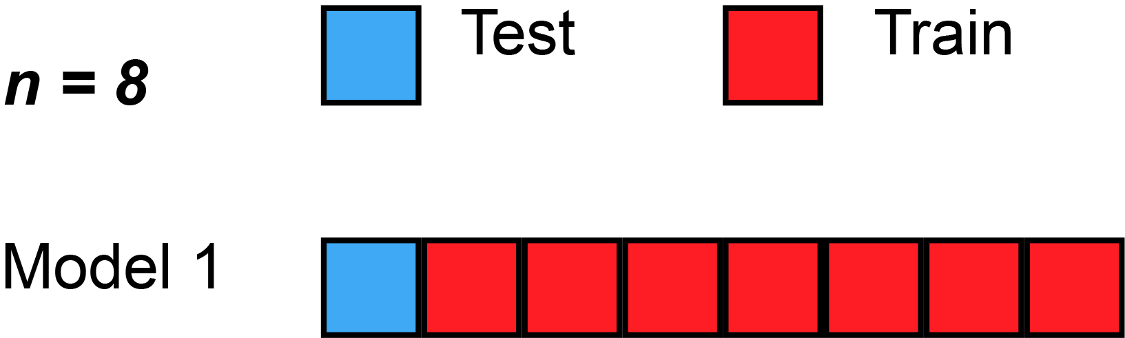
Example of Cross Validation (k=8) where the red and blue square is used respectively as training and validation set
The special case where
A combination of holdout and cross validation can be used when also dealing with a validation set (k-fold cross validation). So after having divided the dataset in a stratify way into training and test set, the training part is again splitted into training and validation set (even in this case with stratify=True).
In a classification scenario, the model can be evaluated by computing different metrics. In order to better understand these metrics could be useful to get some fundamentals:
| Predicted (1) | Predicted (0) | |
|---|---|---|
| Actual (1) | TP | FN |
| Actual (0) | FP | TN |
- True Positive (TP): samples for which the prediction is positive and the true class is positive
- False Positive (FP): samples for which the prediction is positive but the true class is negative
- True Negative (TN): samples for which the prediction is negative and the true class is negative
- False Negative (FN): samples for which the prediction is negative but the true class is positive
Some of the most popular metrics are:
-
Accuracy: ratio of correct predictions over the total number of data points classified
$Accuracy = \frac{#\ correctly\ classified\ samples}{total\ number\ of\ samples\ tested}=\frac{TP+TN}{TP+FP+TN+FN}$ -
Precision: measures the fraction of correct classified instances among the ones classified as positive. Precision is an appropriate measure to use when the aim is to minimize false positives.
$Precision(c) = \frac{#\ samples\ correctly\ assigned\ to\ class\ c}{#\ of\ samples\ assigned\ to\ class\ c}=\frac{TP}{TP+FP}$ -
Recall: it measures how many of the actual positives a model capture through labelling it as True Positive. It is an appropriate score when the aim is to minimize false negatives
$Recall(c) = \frac{#\ samples\ correctly\ assigned\ to\ class\ c}{#\ of\ samples\ actually\ belonging\ to\ c}=\frac{TP}{TP+FN}$ -
F1-score: is the harmonic mean of the precision and recall.
$F1-score(c) = \frac{2\cdot precision(c)\cdot recall(c)}{precision(c) +recall( c)}$
The last three measures are class-specific, and a global metric can be obtained by averaging their values across all classes in the dataset. In particular, class-specific metrics work better when dealing with significantly unbalanced dataset, as they take into account how every class is being learned. Thus, the accuracy measure alone might be misleading in these cases, since may return an high score even if the minority class is not correcly classified.
In this analysis we focus our attention in detecting which customer may be defaults clients, and the positive class captures the attention of the classifier. As already mentioned, in the following section the F1-score will be used to find the best configuration for each model.
Logistic Regression is a parametric, discriminative binary classification algorithm. The name is given after the fact that the algorithm can be interpreted as part of the Generalized Linear Model, where the response variables are distributed according to a Bernoulli distribution. In particular, the model assumes the predictors to be linked to the mean of the response variables (
$ observation\ ( x_{i} , y_{i}) \ ,\ y_{i} \ realization\ of\ Y_{i} \sim Bernoulli( p_{i}( x_{i}))\\ \\ log\left(\frac{p_{i}}{1-p_{i}}\right) =w^{T} x_{i} \ \Longleftrightarrow \ p_{i} =\frac{1}{1+e^{-w^{T} x_{i}}} \ ,\ for\ all\ i $

Logits function
The algorithm then tries to find the MLE (or MAP if a regularization term is added) of the mean of the response variables, by acting on w, assuming i.i.d. samples. Unlike ordinary least squares the optimization problem does not have a closed-form solution, but it’s instead solved through numerical methods.
\begin{equation} \underset{w}{\max} \ \prod ^{n}{i} \ p{i}( x_{i} |w)^{y_{i}} \ *\ ( 1-p_{i}( x_{i} |w))^{1-y_{i}} \end{equation}
A regularization term is often added to prevent the coefficients to reach a too high value which would overfit the training data. The hyperparameter
# C values tuned:
params = {'C': [0.0001, 0.001, 0.01, 0.1, 1, 10]}

#Best configuration found C=0.01
#Data prepocessing: PCA+SMOTE

Tuning of hyperparameter C on the training set both with SMOTE (left) and Cluster Centroids (right) algorithms. Note that scores reported refers to the positive class.
As a result, the output of a Logistic Regression model is the probability of the input sample to be of class 1, hence a confidence measure is also returned when predictions are performed. On top of this, the coefficients returned by the algorithm may give interpretable insights on what attributes are contributing the most to a higher output value, and viceversa.

Coefficients found by Logistic Regression. The PC5 feature empirically gives the highest contribute towards being predicted as defaulters
Decision Trees are the most intuitive and interpretable machine learning model, which predict the target label by learning simple decision rules inferred from the data. At each step, a Decision Tree picks the feature that best divides the space into different labels, by means of the GINI impurity measure:
$ GINI( t) =\sum ^{C}{i=1} p{t}( k)( 1-p_{t}( k)) =1-\sum ^{C}{i=1} p{t}( k)^{2} $
where
A full tree is then constructed on the training data and will be used at classification time for predicting the target label. To avoid overfitting, decision trees are often pruned before reaching their full growth, and predictions are made according to a majority vote on the samples of each leaf. Note how trees cannot handle missing values, but do not suffer from feature scaling since each attribute is treated independently.
# Best configuration found
# Data prepocessing: PCA+SMOTE
params = {'criterion': 'gini', 'max_depth': 5, 'min\_impurity\_decrease': 0.0, 'splitter': 'best'}
Decision trees are however considered weak learners in the majority of cases, and ensemble techniques such as bagging (Random forests) or boosting are in practice applied on them in order to reach higher performances and more robust solutions.
Random Forests are an ensemble method made out of multiple decision trees. Each individual tree in the random forest makes a class prediction and the class with the most votes is assigned to the sample taken into account. The intuition behind this method is that a large number of relatively uncorrelated models (trees) operating as a committee will outperform any of the individual constituent model. Uncorrelation is the key of Random Forests better performances, and this is ensured through two methods:
- Bagging (boostrap aggregation) to promote variance between each internal model, each individual tree is trained on a sample of the same size of the training dataset randomly chosen with replacement;
- In addition, trees are further decorrelated by choosing only a subset of features at each split of each tree (usually
$\sqrt{#features}$ ).
Overall, each tree is then trained on a sample of the same size of the training dataset chosen with replacement, and their splits consider different features every time. This way, even if the decision trees are somewhat overfitting the data and are unstable (high variance), the overall prediction will be statistically more robust (low variance) because of Central Limit Theorem. The prediction is indeed performed by picking the majority class out of all trees.
Hyperparameter tuning on the number of trees and pruning factors for each tree has been performed. In particular, note how the predictions tend to be better as the ensemble model grows horizontally in size:

Tuning of hyperparameter n_estimator is reported both for SMOTE (left) and Cluster Centroids (right) algorithms.
- The choice of the imbalancing technique affect the performance of the Random forest. Indeed, the oversampling technique is preferable.
- Also, the hyperparameter that regulates the number of estimators seems to be irrelevant over the performance of the algorithms.
# Best configuration found
# Data prepocessing: PCA+SMOTE
params = {'criterion': 'gini', 'max_features': 'sqrt', 'n_estimators': 100}
Finally, tree-based model can be used as an alternative method for feature selection. They indeed provide a feature importance measure by means of how much the gini index has been affected on the various splits with the given feature. Compared to decision tree, random forests guarantee robustness and are less prone to overfitting.

Feature importance computed by the random forest on each of the attributes
Support vector machine (SVM) is a parametric linear classification algorithm that aims at separating two classes through a hyperplane in the data dimension. Once the hyperplane has been set, the prediction rule is simply based on whether the test point lays on one side or the other one of it. If more than one hyperplanes fit the purpose, the one with the higher margin (distance) between support vector (the closest points to the hyperplane, one for each class) is selected.
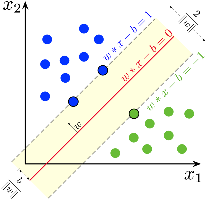
Maximum-margin hyperplane and margins for an SVM trained with samples from two classes. Samples on the margin are called the support vectors.
More formally, it tries to define
$ \underset{w,b}{min} \tfrac{1}{2}\Vert w\Vert ^{2} \ \\ s.t.\ y_{i}\left( w^{T} x_{i} +b\right) \geqslant 1,\ \forall i $
The decision function on a binary label
This model is referred to as Hard-margin SVM, where data is supposed to be linearly separable otherwise no feasible solution would be found.
To extend the model on classes that are not perfectly separable by means of a hyperplane, the hinge loss function is introduced, which penalizes points falling in between the margin:
$ L_{hinge} := \max\left( 0, 1-y_{i}\left( w^{T} x_{i} +b\right)\right) $
The previous opt. problem is then generalized to the soft margin version, which is equivalent to the ERM of the hinge loss with an L2 regularization term:
$ \underset{w,b,\xi }{min} \ \ \tfrac{1}{2}\Vert w\Vert ^{2} \ +C\sum ^{n}{i} \xi {i}\\ \\ s.t.:\\ y{i}\left( w^{T} x{i} +b\right) \geqslant 1-\xi _{i} \ ,\ \forall i\\ \xi _{i} \geqslant 0\ ,\ \forall i\\ $
Where
The Lagrangian Dual Problem is as follows:
Dual Optimization Problem (Soft Margin)
$ \underset{\alpha }{max} \ \ \sum ^{n}_{i} \alpha {i} -\tfrac{1}{2}\sum {i,j} \alpha {i} \alpha {j} y{i} y{j}\left( x^{T}{i} x{j}\right)\\ \\ s.t.: \ \sum \alpha {i} y{i} =0\ \ \land \ 0\leqslant \alpha _{i} \leqslant C,\ \forall i $
By solving the dual problem (e.g. through Quadratic Programming) we find $w=\sum^{n}{i} \alpha{i} y_{i} x_{i}$ as a linear combination of the training data. In particular, only the points that are in between (or exactly on) the margin will have an
Starting from these assumptions, the SVM model can still be generalized to multiclass classification and non-linearly separable classes. Indeed, as for the second case, classes may follow a non-linear pattern and a hyperplane may not be the best fit for explaining our data. However, the given dataset might still be linearly separable when mapped onto a higher-dimensional space by a non-linear function phi, such that the training points are transformed as
While it is possible to compute the SVM algorithm in a higher space through a feature map , a different trick is instead practically used which exploits a nice property of support vector machines. Indeed, note that the dual optimization problem and the newly defined decision function solely depend on the scalar product between the various points at all times. Whenever this property is satisfied then no matter what the higher-dimensional space is, all that it’s needed is a function able to compute the scalar products in the new transformed space.
We then introduce the notion of a Kernel function
for some feature map
Common Kernel functions used are:
- Linear Kernel:
$K( x,x^{\prime} ) =x^{T} x^{\prime}$ - Gaussian RBF Kernel:
$K(x,x^{\prime} )\ =\ \exp (-\gamma \| x-x^{\prime} \| ^{2} ),\ \gamma >0$ - Polynomial Kernel:
$K( x,x^{\prime} ) \ =\ \left( x^{T} x^{\prime} +c\right)^{d}$
In particular, for the Gaussian RBF Kernel the decision function is computing a similarity measure between the test point and the support vectors (weigthed by
The decision function then becomes $sign\left(\sum \alpha {i} y{i}K(x_{i},x)+b\right)$. Finally note that while it is convenient to use a kernel function, the hyperplane in higher space is not actually computed when the kernel trick is applied, i.e. the coefficients of the vector
In this study, both the linear and the gaussian RBF Kernels have been tried. The regularization parameter
#Best configuration found
#polynomial kernel
params = {'C': 100, 'kernel': 'poly'}
#kernel RBF
params = {'C': 1, 'kernel': 'rbf'}| Precision | Recall | F1-score | |
|---|---|---|---|
| SVM POLY + SMOTE | 0.64 | 0.28 | 0.39 |
| SVM RBF + SMOTE | 0.54 | 0.52 | 0.53 |
| SVM POLY + Cluster Centroids | 0.68 | 0.18 | 0.29 |
| SVM RBF + Cluster Centroids | 0.58 | 0.46 | 0.51 |
Scores on validation for the best configuration found with both kernels and both preprocessing techniques
- the score obtained are quite similar indipendently from the preprocessing technique (SMOTE is a little bit better);
- with a polinomial kernel in general the recall on positive class is lower than all the other cases;
- the gaussian version of the SVM outperforms the polinomial one.
In conclusion, also in this case the results should be improved in order to get more accurate prediction on default credit card clients.
The following barplot displays a summary of results in the training-validation phase where all the algorithms are trained with their best hyperparameters (i.e. the ones that maximize the f1-score on positive class), with both techniques presented to overcome class imbalancing problem. 
Comparison of F1-score with different algorithms
- Logistic Regression and Support Vector Machines maintain the same performance regardless the imbalancing techniques used, while this is not true for Random Forest, the reason might be that a decision tree to perform well needs lot of data but at the same time undersampling technique reduce the amount of data.
- Overall, oversampling slightly outperforms undersampling;
- The positive class is the most difficult to classify and none of the models chosen seems to be not able to get the complexity of the problem.
- Empirically has been observed that in general undersampling require more time with respect to oversampling as preprocessing step, this is likely since the first one compute a k-means over all data to find centroids.
All the above mentioned algorithms have been tried out and hypertuned on the training set with a k-fold cross validation technique. The best performing configurations of hyperparameters on the training set have been chosen for rebuilding the models and evaluating them on the test set.
Finally, the table below the results of all the classifiers (in their best configuration) on validation and test set are compared. As we can see, the score obtained on the test set are pretty close to the one obtained in validation.
| Algorithm | Validation Accuracy | Validation F1-score | Test Accuracy | Test F1-score |
|---|---|---|---|---|
| LR + PCA | 0.75 | 0.45 | 0.73 | 0.44 |
| LR + PCA + OS | 0.81 | 0.50 | 0.81 | 0.51 |
| LR + PCA + US | 0.77 | 0.51 | 0.77 | 0.51 |
| RF + PCA | 0.74 | 0.47 | 0.74 | 0.47 |
| RF + PCA + OS | 0.75 | 0.46 | 0.75 | 0.48 |
| RF + PCA + US | 0.47 | 0.38 | 0.47 | 0.37 |
| SVM + PCA | 0.77 | 0.52 | 0.78 | 0.52 |
| SVM + PCA + OS | 0.78 | 0.53 | 0.78 | 0.52 |
| SVM + PCA + US | 0.77 | 0.51 | 0.77 | 0.51 |
LR: Logistic Regression, RF: Random Forest, SVM: Support Vector Machines,
OS: Oversampling (SMOTE), US: Undersampling (Cluster Centroids)
Note that the scores obtained on the test should never be treated as additional information to change how the training is performed, but only as a final evaluation of the model.
In this study different supervised learning algorithms have been inspected and presented with their mathematical details, and finally used on the UCI dataset to build a classification model that is able to predict if a credit card clients will default in the next month. Data preprocessing makes algorithms perform slightly better than when trained with original data: in particular, PCA results are approximately the same, but the computational cost has been lowered. Oversampling and undersampling techniques has been combined with PCA to assess the dataset imbalance problem. Oversampling as mentioned performed slightly better w.r.t. the undersampling, this is likely because the model is trained on a large amount of data. However, all the models implemented achieved comparable results in terms of accuracy.
[1] Default of credit card clients Data Set: UCI dataset link
[2] Yeh, I. C., & Lien, C. H. (2009). The comparisons of data mining techniques for the predictive accuracy of probability of default of credit card clients. Expert Systems with Applications, 36(2), 2473-2480. link
[3] Understanding Machine Learning: From Theory to Algorithms, S. Shalev-Shwartz, S. Ben-David, 2014 link