Mapping Multiple LSTM models on FPGAs

This project includes both the SVD-based approximation algorithms for compressing deep learning models and the FPGA accelerators exploiting such approximation mechanism described in the paper Mapping multiple LSTM models on FPGAs. The accelerators code has been developed in HLS targeting Xilinx FPGAs.

If you plan on using any of the code in this repository, please cite:

@inproceedings{ribes2020mapping,
  title={{Mapping multiple LSTM models on FPGAs}},
  author={Ribes, Stefano and Trancoso, Pedro and Sourdis, Ioannis and Bouganis, Christos-Savvas},
  booktitle={2020 International Conference on Field-Programmable Technology (ICFPT)},
  pages={1--9},
  year={2020},
  organization={IEEE}
}

Disclaimer: The repository is not actively updated and might contain additional experimental features which are not described in the aforementioned paper. Such features might include untested code.

SVD Approximation Algorithm

The following equation indicates the approximation of a single matrix, i.e., LSTM gate, with $R$ rank-1 matrices:

$$\textbf{W}_{\mathrm{M}_j} \approx \sum_{i = 1}^{R} {s_j}^{(i)} \odot \Big( \textbf{u}^{(i)} \cdot {\textbf{v}^{(i)}}^T \Big), \ j = 1, ..., N$$

Our FPGA accelerator's leverages the above equation in its key computation. In fact, it approximates vector-matrix multiplication of the $N$ LSTM inputs with the gate weight matrices, as exemplified in the following equation, which approximates the multiplication between the input vectors $\textbf{x}_j^t$ with the current forget gates weight matrices $\textbf{W}_f^{cur}$.

$$\textbf{x}_j^t \cdot \textbf{W}^{cur}_{f_{j}} \approx \sum_{i = 1}^{R} \big( \textbf{x}_j^t \cdot \textbf{u}^{(i)}_f \big) \cdot {s_f}^{(i)}_j \big) \odot \textbf{v}^{(i)}_f, \ j = 1, ..., N$$

Notice that the vectors $\textbf{u}^{(i)}_f$ and $\textbf{v}^{(i)}_f$ are shared accross the $N$ LSTMs, providing a great compression factor. On top of that, the algorithm also includes a tile-wise pruning scheme to further compress the LSTM weight matrices without impacting their accuracy performance.

The approximation algorithm extracting the SVD components $\textbf{u}^{(i)}$, $s^{(i)}_j$ and $\textbf{v}^{(i)}$ is described in more details in our paper. Its implementation is included in the python folder.

HLS Accelerator Architecture

The accelerator architecture is depicted in the following figure:

It comprises several building blocks. It features custom-made DMA engines for streaming in and out models input-outputs and parameters, e.g., weights. The computational engines are instead organized in SVD kernels, which are responsible of executing the SVD-approximated LSTM models.

SVD Kernels Block Diagram

The inner architecture of each SVD kernel is highlighted as follows:

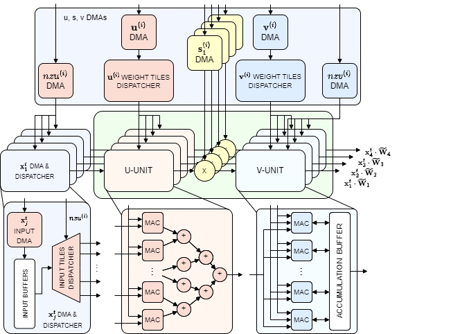
SVD kernels are responsible for the execution of the approximated matrix-vector operation of the LSTM gates mentioned above.

The SVD-kernel is composed of two types of units: U-unit and V-unit. Within the kernel, there are $N$ U-units and $N$ V-units. The U-units are responsible for computing the dot product reported in the following equation:

$$\begin{split} {x_u}_j^{(i)} = \textbf{x}_j^t [{nzu}_k^{(i)}] \cdot \textbf{u}^{(i)} [{nzu}_k^{(i)}], \\\ j = 1, ..., N; \quad k = 1, ..., T_u - ZT_u \end{split}$$

Each U-unit includes $T_u - ZT_u$ parallel multiply-accumulate blocks and an adder tree. In order for the U-units to perform their computation, the $N$ input tiles dispatcher supply the non-pruned input tiles, while the $\textbf{u}^{(i)}$ tile dispatcher broadcasts the non-pruned tiles. Thanks to the list of indexes $nzu$ the $N$ input tiles dispatchers read the input tiles corresponding to the non-pruned tiles of $\textbf{u}^{(i)}$ and then stream them from their on-chip buffers to the respective MACs within the corresponding U-unit.

The $N \times R$ scalars ${x_u}_j^{(i)}$ produced by the U-units are then multiplied by the $s_1^{(i)}, ..., s_j^{(i)}$ scalar components and forwarded to the kernel's V-units as ${x_s}_j^{(i)}$. The V-units perform the operations in the following equation, i.e., the last step of the approximation process:

$$\begin{split} \textbf{x}_j^t \cdot \widetilde{\textbf{W}}_j \approx \sum_{i = 1}^{R} {x_s}_j^{(i)} \odot \textbf{v}^{(i)} [{nzv}_k^{(i)}] \\\ j = 1, ..., N; \quad k = 1, ..., T_v - ZT_v \end{split}$$

Like for the U-units, there is a weight dispatcher which is in charge of supplying the V-unit's MACs with the non-pruned $\textbf{v}^{(i)}$ vector tiles. In order to multiply and accumulate the $x_{s_j}^{(i)}$ scalars with the non-pruned $\textbf{v}^{(i)}$ weight elements, each V-unit utilizes a partitioned accumulation buffer. The buffer is partitioned tile-wise to allow parallel access to it from the MACs.

Finally, the results of the SVD-kernels are streamed to the $\sigma$-kernels for applying the last non-linear functions required by the LSTMs.

Results

We compared our proposed system against two software and two hardware implementations:

• LSTM-SW: Software implementation of baseline LSTM models using GEMV function from OpenBLAS library. Float32 values are used for both activations and weights.
• LSTM-HW: Hardware (FPGA) implementation of baseline LSTM models comprised of 8 parallel 1D systolic arrays for the dense matrix-vector computation, followed by a non-linear unit.
• SVDn-SW: Software implementation of the SVD optimization of the LSTM models that utilizes the same weight values of SVDn-HW before quantization. SVDnSW performs computations on dense weight matrices, despite having many zero values since the OpenBLAS library does not support sparse computation.
• SVD1-HW: A hardware (FPGA) implementation where the mapping of each LSTM model is optimised in isolation.

The baseline implementations without approximation (LSTM-SW and LSTM-HW) are the only ones achieving a 0% accuracy drop. Nevertheless, this is achieved at a high latency, higher than any other design presented. Another expected observation is the fact that all SVDn-SW points have a higher latency than the corresponding SVDn-HW} points. The difference observed ranges between a factor of $3.1\times$ and $5.6\times$.

Another interesting comparison is between the proposed SVDn-HW and the previously proposed SVD1-HW. In particular, it can be observed that the fastest SVDn-HW design is $1.7\times$ faster than the fastest SVD1-HW, considering all plotted points have acceptable accuracy. The most accurate SVDn-HW design has $14\times$ lower accuracy drop than the most accurate SVD1-HW, considering all plotted points have acceptable performance. This is explained by the fact that SVD1-HW applies a similar SVD-based methodology as our approach but does not exploit possible redundancies between weight matrices across LSTM models. As there is a trade-off between accuracy drop and performance, the best SVDn-HW design in the pareto-front is $2\times$ faster and $4.5\times$ more accurate than the best SVD1-HW.

---

Software Requirements

• CMake
• Xilinx Vivado 2018.3 (deprecated)
• Xilinx Vitis 2021.1

CMake Simulation

In order to make CMake include the HLS header libraries, one must modify the file cmake/Modules/FindVitis.cmake.

Windows

"C:\Program Files (x86)\Microsoft Visual Studio 14.0\VC\vcvarsall.bat" amd64
mkdir build
cmake .. -G Ninja
cmake --build . --config Release

Linux

mkdir build
cd build
cmake ..
make -j 4 all

Notes on Using Vitis HLS

AXIS Interface and DMA

Vitis will include the TLAST side channel if and only if TKEEP and TSTRB are also included.

In order to attach the port to a Xilinx DMA, the TLAST signal must be properly set HIGH at the end of the data transmission.

The TKEEP and TSTRB signals must be always set to HIGH, as indicated in the AXIS documentation.

Note: for using external DMAs, we need the TLAST, TKEEP and TSTRB signals. In particular, TKEEP and TSTRB must be all set (i.e. all ones) in order to signal data packets.

AxiStreamInterface Class

This repository contains a wrapper class for kernel arguments of type hls::stream named AxiStreamInterface. The class is implemented following a Policy-based C++ paradigm, meaning that it accepts either a AxiStreamPort or AxiStreamFifo as possible policies (in practice, a template argument).

The idea is to have a kernel argument, i.e. an HLS port, which can be either an AXIS interface with side-channels, or a bare FIFO interface connected to another kernel. In fact, Vitis HLS doesn't allow stream interfaces with side-channels within an IP. To overcome this issue, the AxiStreamInterface can be customized to be an IP port or a FIFO port, depending on the use of the kernel.

An example of this can be seen in HlsKernelU and in svd::SvdKernel, which specialize the svd::KernelU function template. In the first case, the svd::KernelU has its output stream port xu_port connected to one of the IP's ports (with side-channels). In the latter case instead, svd::KernelU is connected to svd::KernelS, and so its xu_port argument is an internal FIFO (without side-channels).

The AxiStreamInterface class in axis_lib.h can also be used with hls::vector types.

AXIS Interfaces and depth

In order to implement AXIS interfaces, avoid using depth in the pragma, as follows:

const int kAxiBitwidth = 128;

void HlsVectorKernelU(hls::stream<ap_axiu<kAxiBitwidth, 0, 0, 0> >& x_port,
                      hls::stream<ap_axiu<kAxiBitwidth, 0, 0, 0> >& y_port) {
#pragma HLS INTERFACE axis port=x_port // depth=... <- DON'T SPECIFY THE DEPTH!
#pragma HLS INTERFACE axis port=y_port // depth=... <- DON'T SPECIFY THE DEPTH!
	// ...
}

The type ap_axiu must now be used to generate AXIS with side channels.

hls::vector Arrays on AXI-Lite Interfaces

In Vitis 2021.1 it is not allowed to have hls::vector type arguments mapped to AXI-Lite interfaces. Instead, use bare arrays, e.g. const int x[N] instead of const hls::vector<int, N> x.

Partitioning hls::vector Arrays

A standard way of partitioning an array is:

  hls::stream<hls::vector<int, 4> > x_streams[M][N];
#pragma HLS ARRAY_PARTITION variable=x_streams complete dim=0

However, since we are dealing with a hls::vector type, setting dim=0 (all dimensions) will partition the array on the vector dimension too.

In the example above, Vitis will create M * N * 4 different streams (instead of just M * N). To fix it, manually specify the partitioning on the dimensions, like so:

  hls::stream<hls::vector<int, 4> > x_streams[M][N];
#pragma HLS ARRAY_PARTITION variable=x_streams complete dim=1
#pragma HLS ARRAY_PARTITION variable=x_streams complete dim=2

HLS Vector Patch

If the project will be compiled with the Vitis HLS libraries, it needs a patch in the hls::vector class.

Simply add the following line in the vector class after the public: statement:

public:
  static const int width = N;

In this way, one can access the number of elements in a hls::vector at compile/synthesis time by doing:

hls::vector<int, 5> a;
std::cout << "Number of elements in a: " << a::width << std::endl;

// > Number of elements in a: 5