![]()


This REANA reproducible analysis example emulates a typical particle physics analysis where the signal and background data is processed and fitted against a model. The example will use the RooFit package of the ROOT framework.
Making a research data analysis reproducible basically means to provide "runnable recipes" addressing (1) where is the input data, (2) what software was used to analyse the data, (3) which computing environments were used to run the software and (4) which computational workflow steps were taken to run the analysis. This will permit to instantiate the analysis on the computational cloud and run the analysis to obtain (5) output results.
In this example, the signal and background data will be generated; see below. Therefore there is no explicit input file to be taken care of.
The analysis will consist of two stages. In the first stage, signal and background are generated. In the second stage, a fit will be made for the signal and background.
For the first generation stage, gendata.C is a ROOT macro that generates signal and background data.
For the second fitting stage, fitdata.C is a ROOT macro that makes a fit for the signal and the background data.
The code was taken from the RooFit tutorial rf502_wspacewrite.C and was slightly modified.
In order to be able to rerun the analysis even several years in the future, we need to "encapsulate the current compute environment", for example to freeze the ROOT version our analysis is using. We shall achieve this by preparing a Docker container image for our analysis steps.
This analysis example is runs within the ROOT6 analysis framework. The computing environment can be therefore easily encapsulated by using the upstream reana-env-root6 base image. (See there how it was created.)
We shall use the ROOT version 6.18.04. Note that we can actually use this container image
"as is", because our two macros gendata.C and fitdata.C can be "uploaded" and
"mounted" into the running container at runtime. There is no need to compile any of the
analysis source code beforehand. We can therefore use the ROOT 6.18.04 base image
directly, without building a new container image specially dedicated to our analysis. The
ROOT 6.18.04 base image fully specifies the complete analysis environment that we need
for our analysis.
The analysis workflow is simple and consists of two above-mentioned stages:
           START
            |
            |
            V
+-------------------------+
| (1) generate data       |
|                         |
|    $ root gendata.C ... |
+-------------------------+
            |
            | data.root
            V
+-------------------------+
| (2) fit data            |
|                         |
|    $ root fitdata.C ... |
+-------------------------+
            |
            | plot.png
            V
           STOP
For example:
$ root -b -q 'gendata.C(20000,"data.root")'
$ root -b -q 'fitdata.C("data.root","plot.png")'
$ ls -l plot.png
Note that you can also use CWL, Yadage or Snakemake workflow specifications:
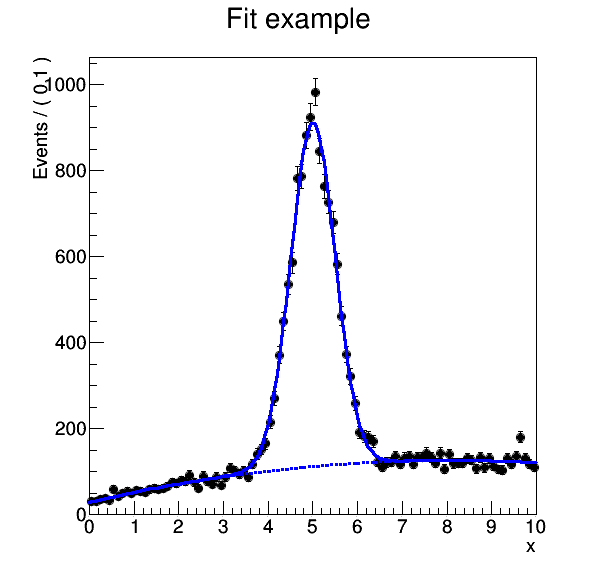
The example produces a plot where the signal and background data is fitted against the model:
There are two ways to execute this analysis example on REANA.
If you would like to simply launch this analysis example on the REANA instance at CERN and inspect its results using the web interface, please click on one of the following badges, depending on which workflow system (CWL, Serial, Snakemake, Yadage) you would like to use:


If you would like a step-by-step guide on how to use the REANA command-line client to launch this analysis example, please read on.
We start by creating a reana.yaml file describing the above analysis structure with its inputs, code, runtime environment, computational workflow steps and expected outputs:
version: 0.6.0
inputs:
  files:
    - code/gendata.C
    - code/fitdata.C
  parameters:
    events: 20000
    data: results/data.root
    plot: results/plot.png
workflow:
  type: serial
  specification:
    steps:
      - name: gendata
        environment: 'docker.io/reanahub/reana-env-root6:6.18.04'
        commands:
        - mkdir -p results && root -b -q 'code/gendata.C(${events},"${data}")'
      - name: fitdata
        environment: 'docker.io/reanahub/reana-env-root6:6.18.04'
        commands:
        - root -b -q 'code/fitdata.C("${data}","${plot}")'
outputs:
  files:
    - results/plot.png
In this example we are using a simple Serial workflow engine to represent our sequential computational workflow steps. Note that we can also use the CWL workflow specification (see reana-cwl.yaml), the Yadage workflow specification (see reana-yadage.yaml) or the Snakemake workflow specification (see reana-snakemake.yaml).
We can now install the REANA command-line client, run the analysis and download the resulting plots:
$ # create new virtual environment
$ virtualenv ~/.virtualenvs/reana
$ source ~/.virtualenvs/reana/bin/activate
$ # install REANA client
$ pip install reana-client
$ # connect to some REANA cloud instance
$ export REANA_SERVER_URL=https://reana.cern.ch/
$ export REANA_ACCESS_TOKEN=XXXXXXX
$ # create new workflow
$ reana-client create -n myanalysis
$ export REANA_WORKON=myanalysis
$ # upload input code, data and workflow to the workspace
$ reana-client upload
$ # start computational workflow
$ reana-client start
$ # ... should be finished in about a minute
$ reana-client status
$ # list workspace files
$ reana-client ls
$ # download output results
$ reana-client download
Please see the REANA-Client documentation for
more detailed explanation of typical reana-client usage scenarios.