Theoretical Introduction
This tutorial provides a short introduction to multivariate transfer entropy (mTE) estimation. Wherever possible, we point to the literature for a more in-depth treatment of the topics discussed. For code examples see the tutorial section in the Wiki.
IDTxl expects an input data set consisting of samples (i.e., observations or realisations) of at least two processes. IDTxl provides a flexible data structure which is compatible with different experimental/theoretical scenarios:
- samples can be collected over time as a time series;
- multiple replications of a single sample can be collected (a replication is intended as a physical or temporal copy of the process, or a single experimental trial);
- samples can be collected both over time and over replications to form an ensemble of time series, which is treated as a 3D structure. (See also Wollstadt, 2014, PLOS 9(7) and Gomez-Herrero, 2015, Entropy for details on the estimation of TE from ensembles of time series.)
At the current stage, we assume that each process is sampled at discrete time steps and using the same sampling rate.
For any given target process, the goal of mTE estimation is to infer the set of source processes in the network (also denoted as 'parent' processes) that collectively contribute to the computation of the target's next state. These sources are defined as relevant for the target.
TE quantifies the amount of information (i.e. the reduction of uncertainty) that the past of a source process X provides about the current value of a target process Yn, in the context of Y's own past. In a multivariate setting, a set of sources X={Xi, i=1,...,M} is provided. We define the mTE from Xi to Y as the information that the past of Xi provides about Yn, in the context of both Y's past and all the other relevant sources in X. The challenge is then to define and identify the relevant sources. In principle, the mTE from Xi to Y could be computed by conditioning on all the other sources in the network, i.e., X \ Xi. However, in practice, the size of the conditioning set must be reduced in order to reduce the dimensionality of the problem (also described as tackling the 'curse of dimensionality'). The idea is to restrict the conditioning set by finding and including the 'relevant' sources only (i.e., the sources that participate with Xi in reducing the uncertainty about Yn, in the context of Y's own past) . The set of relevant sources will be denoted as Z.
How to infer Z from X ? A brute force algorithm would require to test all the 2|X| subsets of X for optimality, which is intractable even for a small number of sources. Instead, IDTxl employs a greedy algorithm and iteratively builds Z by maximising a conditional mutual information criterion: first, a set of candidate variables c ∈ C is defined from the pasts of the sources X; then, Z is built by iteratively including the candidate variables c that provides statistically-significant, maximum information about the current value Yn, conditioned on all the variables that have already been selected. More formally: at each iteration, the algorithm selects the past variable c ∈ C that maximises the conditional mutual information I(c ; Yn | Z) and passes a statistical significance test (more on the statistical tests below). The set of selected variables forms a multivariate, non-uniform embedding of X (Faes, 2011, Phys. Rev. E).
The candidate set of past variables C is defined by the user by providing the maximum lag parameter for the target and for the sources. The maximum lag restricts the number of past variables in the target and sources time-series that are tested for inclusion in Z. Importantly, IDTxl tests the variables from the target's past first, before testing the variables from the sources' past1. In the figure below, l3 denotes the maximum lag for the sources' past, l1 the minimum lag for the sources' past, and l2 is the maximum lag for the target's past:
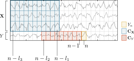
The minimum lag for the target is always set to 1 sample to ensure self-prediction optimality (Wibral, 2013, PLOS 8(2)).
Note that IDTxl requires no further parameters beyond the max lags and the parameters for statistical testing (estimator type, number of permutations, and critical alpha level). Statistical significance provides an adaptive stopping criterion for parents selection. Statistical testing of the estimated conditional mutual information is necessary to assess whether the estimated value is significantly different from zero: non-zero estimates may occur for independent variables due to the finite number of samples and the estimator bias (see also Vicente, 2011, J. Comp. Neurosci., 20(1) and Kraskov, 2004, Phys. Rev. E 69(6)).
Currently, for estimating (conditional) mutual information information from continuous data a Gaussian as well as the Kraskov-Stögbaur-Grassberger estimator Kraskov, 2004, Phys. Rev. E 69(6) are implemented. For discrete data, a plug-in estimator is used (e.g., Hlavackova-Schindler, 2007, Phys. Report, 441). See the tutorial page CMI estimators for further details on available estimators.
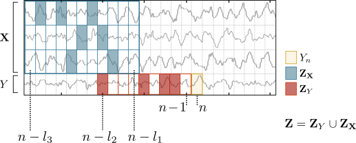
An example of a possible embedding Z returned by the algorithm is shown in the figure below (filled rectangles indicate selected variables):
The greedy algorithm operates in five steps:
-
Initialise Z as an empty set and consider the candidate sets for Y's past (CY) and X's past (CX).
-
Select variables from CY1:
- For each candidate, c ∈ CY, estimate the information contribution to Yn as I(c ; Yn | Z)
- Find the candidate with maximum information contribution, c*, and perform a significance test2; if significant, add c* to Z and remove it from CY. We use the maximum statistic to test for significance while controlling the FWER (family-wise error rate).
- Terminate if I(c* ; Yn | Z) is not significant or CY is empty.
-
Select variables from X's past (i.e., from CX):
- Iteratively test candidates in CX following the procedure described in step 2.
-
Prune Z: Test and remove redundant variables in Z using the minimum statistic. The minimum statistic computes the conditional mutual information between every selected variable in Z and the current value, conditional on all the remaining variables in Z. This test is performed to ensure that the variables included in the early steps of the iteration still provide a statistically-significant information contribution in the context of the final parent set Z. See Lizier, 2012, Max Planck Preprint No. 25.
-
Perform statistical tests on the final set Z:
- Perform an omnibus test to test the collective information transfer from all the relevant (informative) source variables to the target: I(ZX ; Yn |ZY ). The resulting omnibus p-value is later used for correction of the FWER at the network level.
- If the omnibus test is significant, perform a sequential maximum statistic on each selected variable z ∈ Z to obtain each variable's final information contribution and p-value
Finally, the mTE between a single source Xi and target Y can be computed from the inferred non-uniform embedding Z: collect from Z all of Xi's selected past variables, Xi, and calculate the mTE as I(Xi ; Yn | Z\Xi). Note that time lag between Xi's selected past variables and the current value at time n indicates the information-transfer delay (Wibral, 2013, PLOS 8(2)). The delay can be estimated as the lag of the past variable which provides the maximum individual information contribution (the maximum contribution is indicated either by the maximum raw TE estimate or by the minimum p-value over all variables from that source).
Repeat the greedy algorithm for each node in the network. For theoretical and some practical runtimes, see the Runtimes and Benchmarking page.
Note further that the proposed approach to multivariate TE estimation is sometimes also termed conditional transfer entropy Bossomaier, 2016.
The maximum statistic is used to test the information contribution of a candidate variable to the target's current value. The maximum statistic mirrors the greedy selection process and is used to control the FWER when selecting the relevant past variables to include in Z. The statistic works as follows:
Assume we have picked the candidate variable c* (from the set of candidates C) which provides the maximum information contribution to the target, i.e., I(c* ; Yn | Z). The following algorithm is used to test I(c* ; Yn | Z) for statistical significance:
- for each c ∈ C, generate a surrogate time-series c' and calculate I(c' ; Yn |Z)
- pick the maximum surrogate value I(c' ; Yn |Z) among all surrogate estimates
- repeat steps 1 and 2 a sufficient3 number of times to obtain a distribution of maximum surrogate values
- calculate a p-value for c* as the fraction of surrogate values larger than I(c* ; Yn | Z) and compare against the critical alpha-level.
Note that surrogate distributions can be derived analytically for Gaussian estimators, so that steps 1-3 can be omitted.
The minimum statistic is used to prune the set of selected source candidates, ZX, after the inclusion of the candidates has terminated. The pruning step removes the selected variables that have become redundant in the context of the final set Z. The minimum statistic works similarly to the maximum statistic:
Assume we have picked the selected variable z* from ZX that has minimum information contribution I(z* ; Yn | Z\z*). The following algorithm is used to test if I(z* ; Yn | Z\z*) is still significant in the context of Z:
- for each z ∈ ZX, generate a surrogate time-series z' and calculate I(z' ; Yn |Z\z*)
- pick the minimum estimate I(z' ; Yn |Z\z*) among all surrogate estimates
- repeat steps 1 and 2 a sufficient number of times to obtain a distribution of minimum surrogate values
- calculate a p-value for z* as the fraction of surrogate values that is larger than I(z* ; Yn | Z\z*) and compare against the critical alpha-level.
Note that surrogate distributions can be derived analytically for Gaussian estimators, so that steps 1-3 can be omitted.
The omnibus test is used to test the total information transfer from all the selected source variables, ZX, to the target Yn:
- permute realisations of Yn to obtain Y'n and calculate I(ZX ; Y'n | ZY)
- repeat step 1 a sufficient number of times
- calculate the omnibus p-value as the fraction of surrogate values larger than I(ZX ; Yn | ZY) and compare against the critical alpha-level.
Note that surrogate distributions can be derived analytically for Gaussian estimators, so that steps 1-2 can be omitted. The omnibus test's p-value is used to control the FWER at the level of links in the network via FDR-correction (Benjamini et al. (1995)).
If the omnibus test finds significant total information transfer, I(ZX ; Yn | ZY), into the target, the sequential maximum statistic tests each selected source variable in the final set ZX. The sequential maximum statistic works similarly to the maximum statistic. The difference is that the surrogate values are ordered by magnitude, which results in a distribution of maximum values, a distribution of second-largest values, a distribution of third-largest values, and so forth. The selected variables are sorted by their individual information contribution. The variable with the largest information contribution is compared against the maximum distribution, the variable with the second-largest contribution against the second-largest distribution, and so forth. As soon as a variable is no longer significant compared to its surrogate distribution of equal rank, that variable and all the other variables of lower rank are removed from the candidate set.
1 We first find all relevant variables in the target's own past; otherwise, the information from the sources' pasts may be overestimated later (see Wibral, 2013, PLOS 8(2) for a discussion of this self-prediction optimality). Moreover, this approach is consistent with the distributed-computation modelling framework, whereby the information storage is computed first, followed by the information transfer.
2 In IDTxl, statistical testing of estimated quantities is usually carried out by performing a test against a distribution estimated from surrogate data. The distribution is obtained by first permuting data to obtain surrogate data, and second re-estimating the quantity from surrogate data. This is repeated a sufficient number of times to obtain a test-distribution of estimates from surrogate data. The original estimate is then compared against this distribution. A p-value is obtained as the fraction of surrogate estimates that are more extreme than the original estimate. If an estimator with a known test-distribution is used (e.g., Gaussian), surrogate estimates can be created analytically to save computing time.
3 The number of permutations is considered sufficient if it theoretically allows obtaining a p-value that is smaller than the critical alpha-level. The p-value is calculated as the fraction of surrogate values larger than the tested quantity. In the most extreme case, where no surrogate value is larger, the p-value is calculated as (1/number of permutations). This is the lowest obtainable p-value in the test. If the critical alpha level is lower than (1/number of permutations), the test can never return a significant result. Hence, the number of permutations and critical alpha-level should be set such that alpha > 1/no. permutations.
As an example of mTE estimation, consider the following toy network, where nodes represent (stochastic) processes and arrows represent interactions between processes:
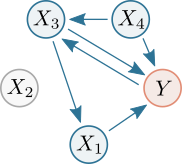
Let Y be the current target of interest. Nodes highlighted in blue represent the set of relevant sources Z={X1, X3, X4}, i.e. the sources that contribute to the target's current value Yn.
Estimating the mTE into the target Y requires inferring the set Z containing the relevant sources (or parents) of Y. Once Z is inferred, we can compute the mTE from a single process into the target as a conditional transfer entropy, which accounts for the potential effects of the remaining relevant sources. Formally, the mTE from a single source (e.g., X3) into Y is defined as the TE from X3 to Y, conditioned on Z and excluding X3:

In order to infer mTE for each source-target pair in the network, the process of mTE estimation is repeated for each node in the network, i.e., the algorithm iteratively treats each node in the network as the current target and infers its relevant sources in the network.
In addition to mTE, IDTxl implements further algorithms for network inference. In the beginning, we assumed a multivariate setting with a single target process, Y, and a set of source process, X. We defined the mTE from a source Xi to Y as the information the past of Xi provides about Yn, in the context of both Y's past and the past of all other relevant sources in X. We used the described greedy approach to build the set, Z, of relevant past variables. We now additionally define
- bivariate transfer entropy (bTE) as the information the past of a single source X provides about about Yn in the context of Yn’s past alone;
- bivariate mutual information (bMI) as the information the past of a single source X provides about about Yn without considering Yn’s past;
- multivariate mutual information (mMI) as the information the past of a single source Xi provides about about Yn in the context of all the other relevant sources in X, without considering Yn’s past.
IDTxl provides algorithms to estimate these quantitites. The algorithms use the described greedy strategy to build a non-uniform embedding from the respective candidates with the goal to maximise the information the set of selected variables, Z, has about Yn. The algorithms use the maximum statistic to determine whether a variable provides statistically significant information about Yn in the inclusion step. Then the algorithms use the minimum statistic to prune the set of selected variables. The final set Z of selected variables is then tested using the omnibus test and sequential maximum statistics. See also the documentation and the tutorials for further details.