Simple two-pole equalizer with variable oversampling.
| Latest release: | v.1.2.2 |
|---|---|
| Latest development: | Formats: |
| VST3, Standalone | |
| LV2, VST3, Standalone | |
| AU, VST3, Standalone | |
| AU, VST3, Standalone |
Verified by Pluginval
Created with the StoneyDSP C++ library for JUCE
![]()
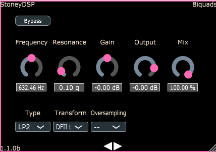
Multi-mode Biquad filter for audio analysis purposes using variable BiLinear transforms, processing precision, and oversampling to achieve high-quality results.
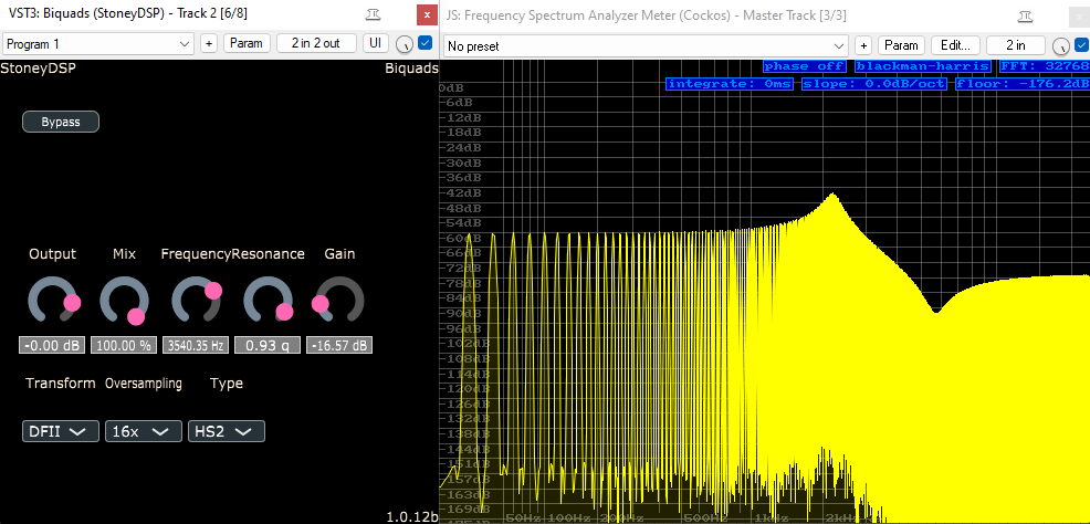
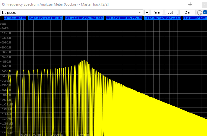
(Shown below; a resonant 2-pole Low Shelf filter with high oversampling, performed on a harmonic-rich 20Hz band-limited Impulse Response in Reaper)
- Implementing various 6dB- and 12dB- filter types (such as low pass, high pass, band pass, shelves, plus many more) using variable BiLinear transforms, switchable processing precision, and oversampling to achieve high-quality results (much more to come)!
- This filter is subject to amplitude and phase warping of the frequency spectrum approaching the Nyquist frequency when oversampling is not used.
- There is parameter smoothing on the Frequency, Resonance, and Gain controls - however, BE AWARE that modulating parameters in real-time WILL create loud clicks and pops while passing audio under certain settings, such as Direct Form I (read on for more).
- IO - Toggles the filter band on or off.
- Frequency - Sets the centre frequency of the equalizer filter.
- Resonance - Increases the amount of "emphasis" of the corner frequency
- Gain - Boost/cut the audio at the centre frequency (affects only the Peak and Shelf modes!)
- Type* - Chooses the type of filter to use. See below for more.
- Transform** - Chooses the type of bilinear transform to use. See below for more.
- Oversampling - Increasing the oversampling will improve performance at high frequencies - at the cost of more CPU!
- Mix - Blend between the filter affect (100%) and the dry signal (0%).
- Precision - Switch between Float precision (High Quality) and Double precision (beyond High Quality) in the audio path
- Bypass - Toggles the entire plugin on or off.
Type*;
Available filter types -
- Low Pass (2) - 2nd order Low Pass filter with variable resonance
- Low Pass (1) - 1st order Low Pass filter
- High Pass (2) - 2nd order High Pass filter with variable resonance
- High Pass (1) - 1st order Low Pass filter
- Band Pass (2) - 2nd order Band Pass filter with variable resonance
- Band Pass (2c) - 2nd order Band Pass filter with variable resonance and compensated gain
- Peak (2) - 2nd order Peak filter
- Notch (2) - 2nd order Notch filter
- All Pass (2) - 2nd order All Pass filter
- Low Shelf (2) - 2nd order Low Shelf filter with variable resonance
- Low Shelf (1) - 1st order Low Shelf filter with compensated corner frequency
- Low Shelf (1c) - 1st order Low Shelf filter
- High Shelf (2) - 2nd order High Shelf filter with variable resonance
- High Shelf (1) - 1st order High Shelf filter with compensated corner frequency
- High Shelf (1c) - 1st order High Shelf filter
Transform**;
Four different ways of applying the filter to the audio.
- Direct Form I
- Direct Form II
- Direct Form I transposed
- Direct Form II transposed
For further information, please continue reading.
In realising this digital biquad equalizer design, we shall come to see that the entire equalizer system is really just a "gain" system - the audio enters, gets split into several "copies", and these copies are all re-applied back to the original audio stream at variying levels of gain - and, in many cases, with their sign flipped (i.e., polarity inversed). The output of our system will be the final product of these calculations.
Before we look at these so-say "simple" gain functions that happen inside the system more closely, first, let's familiarize ourselves with some terminology and core concepts.
In the system we described above, we mentioned that our frequency equalizer is internally really just a system of various "gains" applied to the input signal. How so?
Let's start by thinking of our audio stream entering our "system" and coming out the other side, unchanged. Here's some basic pseudo-code describing this scenario:
{
	x = input sample;

	y = x;

	output sample = y;
}
Since the system described above doesn't actually "do anything", it isn't currently useful. Let's build toward the "gain system" described earlier, by introducing the idea of "coefficients" - these coefficient objects are just simple numerical values that represent the amount of gain to apply at a particular point in our system.
Traditionally speaking, we have two types of "coefficient" objects;
- Numerator
- Denominator
Furthermore, we shall refer to our "Numerator" coefficient object as "b", while our "Denonimator" shall be "a". Please note: these labels are occasionally swapped over in some literatures!
Let's take our crude metal-box-with-wire system, and begin applying the gains, i.e., our "coefficient" objects, in a simple fashion. As stated above, we have one "numerator" coefficient named "b", and a "denominator" coefficient named "a". Here is a simple expression to give you the idea of what these two initial coefficients do for our input audio sample:
{
    x = input sample;

    b = 1;
    a = 1;

    y = x * b;

    output sample = y;
}
Coefficient "b" is used as a gain multiplier for our direct signal (i.e., the level of our input signal to appear at the output).
But first, our "a" is used to scale (multiply) our "b" like so:
{
    x = input sample;

    a = 1;
    b = 1;

    y = x * (b * (1/a));

    output sample = y;
}
In fact, what we shall see moving forward, is that our initial coefficient "a" is something of a special case; it is used as a gain multiplier for all coefficients except for itself. That is, all other coefficients except for a, are multiplied by 1/a = 1.
So that the above pseudo-code and the below are equivalent:
{
    x = input sample;

    a = 1;
    b = 1/a;

    y = x * b;

    output sample = y;
}
The key difference in the above example, is that we see how "a" only works directly on "b", and thus only ever indirectly on "x".
The expressions are of course mathematically equivalent, but the above version explicitly demomstrates the concept that "all other coefficients except for a, are multiplied by 1/a = 1" that we'd just outlined previously.
note: It is extremely common to see this initial "denominator" coefficient, "a", "normalised" to a value of 1, or even disregarded entirely, in most literature and implementations (since it is assumed that we always want our coefficients to be their actual values, instead of being scaled by 1/something else). This does help to keep things more simple. Doing so, however, does close down some potentially worthwhile experiments for much later on when addressing the topic of "de-cramping" a digital equalizer.
Our implementations shall maintain that "b" = numerator, "a" = denominator, and that our intial "a" is a valid parameter in our calculations, while still keeping things as simple as possible.
So, for all of the above, we've still only got a crude metal box containing a single wire... except, we've now stuck a potentiometer on the front, which controls the gain of said wire; this pot has a label saying "b".
We've also stuck a second potentiometer on the front, this one labelled "a", and which controls the gain of "b", and is wired in an inverse fashion.
Actually, both of these pots are infact bi-polar. That is, at centre detent, each potentiometer outputs a voltage of 0v. And;
- When fully clockwise, "b" outputs a voltage of 1v. When fully counter-clockwise, it's output is -1v.
- The pot labelled "a" is the opposite; clockwise gives -1v, and counter-clockwise gives us 1v. (this inversion is the result of the 1/a in it's path).
In our metal-box-with-two-pots "system" so far, we already know that "b" is actually = b * (1/a).
Potentiometer "a" does not touch the input signal itself, it's just connected to the "b" pot, as above.
And yet it's still just a simple volume control overall, now with a silly interface; not really anything approaching our desired equalizer system. We only have one connection (input-to-output) to interact with, so how can we add more?
At this point we introduce the traditional concepts of "feedback" into our system. We likely all know what this means in at least some context: the input of a system is fed some amount of it's own output.
This is of course a notorious way to introduce chaos, near-unpredictability, and deafening/damaging results to an audio system. Let's call such a case "positive feedback" - the changed output is being fed back into it's own input, thus the system iterates over itself infinitely (until some part of the chain reaches it's operating limit and explodes).
Here's a very simplified pseudo-version of the "positive feedback" idea:
{
    x = input sample;

    y = x + y;

    output sample = y;
}
That's right - we're adding "y" to itself. So that if "x" = 0.7, and "y" = 0.9, technically "y" would also be equal to x + y = 1.6, but if that were the case then "y" would also be equal to x + y = 2.5, and so on... all in the same instant. Potentially, our signal could grow indefinitely... and dangerously.
And what of "negative feedback"? What's the difference?
{
    x = input sample;

    y = x - y;

    output sample = y;
}
So now, if as before "x" = 0.7, and "y" = 0.9, "y" should also be equal to -0.2, but also 0.9, and thus equal to -0.2... and so on. The subtraction in this case produces a stable system, that we can see "oscillates" from one value to another and back.
Due to the bi-polar nature of both our input signal and our coefficients, it is also worth considering an additional case; Adding a negative number to a positive number.
For example, if "y" = -0.9, and were added to "x" = 0.7, the resultant addition is equivalant to subtracting "y" - if "y" were a positive number.
Thus, we can always invert the sign of any of our coefficients (or input signal), and always sum our results (addition) instead of having to chain additions and subtractions together, later on.
But, how can this be? How can "y" know itself instantaneously, if it is continually changing based on it's own input-output relationship?
Such is the case when working with feedback. Fortunately (at least for this write up), our digital system is bound by the sampling theorem, in which the closest thing we have to "near-instant" in such a calculation is one audio sample. This will be investigated - utilized, even - later on in our design.
Let's revert to allowing our input signal to pass to the output, scaled by b * (1/a) as before:
{
    x = input sample;

    a = 1;
    b = 1/a;

    y = x * b;

    output sample = y;
}
As we know, the above is a just crude metal box with two holes, one wire, and two labelled pots; literally a "gain multiplier of a gain multiplier", nothing more.
In order to do anything more interesting with it, we will need more "degrees of freedom" to work with.
We also know that beyond a basic gain multiplication, we can also manipulate the signal via the use of feedback - wherein the system's input is detecting it's own output.
In order to include "more degrees of freedom" in our system, we can consider using combinations of gain and feedback - both in both positive, and negative, applications.
We shall expand our system's current parameter set, the coefficients, by double. Let's introduce numbers:
- b0 = gain of input signal (exactly as our previous "b")
- a0 = scalar of coefficients (to be used as 1/a0, exactly as our previous "a")
And the new terms:
- b1 = positive feedback path
- a1 = negative feedback path
Giving us a total of four "degrees of freedom" with which to manipulate our input signal.
We can still start off by passing our audio directly, but with the new coefficients wired into place - we simply set them to 0 for now:
{
    x = input sample;

    a0 = 1;
    b0 = 1/a0;

    a1 = 0/a0;
    b1 = 0/a0;

    y = ((x * b0) + (x * b1) + (y * a1));

    output sample = y;
}
So, if;
a0 = 1;

// This one is often left out of the literature...
1/a0 = 1;
Therefore;
// input signal multiplier...
b0 = 1;

// negative feedback signal multiplier...
a1 = 0;

// positive feedback signal multiplier...
b1 = 0;
Thus for "y";
y = (x * 1) + 0 + 0;
Or rather:
y = x;
So, nothing has so far changed, except we've now got two more potentiometers on the front of our metal box; one labelled "b1", and another labelled "a1".
I have some very interesting experiments in which I have exposed these coefficients on the GUI of an audio plugin, allowing the user to play with them directly. The results are certainly interesting, and do in fact sometimes go beyond typically-expected filter shapes (for a one-pole system) - however, the main take-away from testing that plugin, is that the results are entirely unpredictable (being a feedback system) and that a typical filter implementation, even a most basic one (read on), will instead use a more generic parameter (such as a "frequency" knob) to update several coefficients simultaneously.
The test plugin described above, and concurrent write-up, may appear on the writers' Github at some point in the near future - this section will updated with links if so.
For now, we have described a system that has an input, an output, and four pots that behave and interact in unpredictable and potentially hazardous ways.
Meanwhile, how can we utilize our system's new "degrees of freedom" to create something greater than a volume control? And how to do this in a controlled, and controllable, fashion?
For now, let's begin at the beginning.
- 1st-order Low Pass Filter
{
    b0 = ⍵ / (1 + ⍵);
    b1 = ⍵ / (1 + ⍵);
    a0 = 1;
    a1 = -1 * ((1 - ⍵) / (1 + ⍵));
}
In the above pseudo-code, we are shown a formula for manipulating our coefficients to provide us a simple 1st-order (i.e., 1 pole, 1 zero) Low Pass Filter. The writer shall assume the reader is familiar with this filter concept in usage terms, and is more interested in the DSP.
At this point, we have reasonably concluded that our system itself required more "degrees of freedom" in order to produce interesting and useful results, but that user exposure to all of this freedom leads to screeching feedback or complete silence at literally every turn of it's four pots.
Instead of this array of potential disasters, the above formula presents a classical way to manipulate three out of four coefficients, all at the same time, by using just a single parameter acting them all.
Our value "⍵" ("omega"), is this new parameter. As the value of "⍵" changes, so does the centre frequency (the writer refers to the -3dB point as centre frequency) of the filter. So with this formula, we have infact retained our "degrees of freedom", yet restricted user input to a much more simple, sensible, singular control parameter; one pot which, as it turns clockwise, the centre frequency increases.
To demonstrate that we have infact retained (and exponentially increased) our "degrees of freedom", let's perform a sort of inversion of this formula but retain the simple one-control function of it:
- 1st-order High Pass Filter
{
	b0 = 1 / (1 + ⍵);
	b1 = (1 / (1 + ⍵)) * -1;
	a0 = 1;
	a1 = ((1 - ⍵) / (1 + ⍵)) * -1;
}
We can notice, even at a glance, that these two formulas are effectively the inverse of one another - as are the filter responses! Our Low Pass is transformed into a High Pass by this numerical inversion.
As we explore further filter types and orders, we will want to formalize a control system that correctly maps as few user-parameters as possible, to the coefficients, using corrected scaling (for Sample Rate changes, as an example) to provide a predictable result under all settings.
- ⍵ = omega
- ⍺ = alpha
- A = gain (only used in peaking and shelving filter calculations!)
{
    ⍵ = frequencyParameter * (2π / sampleRate);
    sin(θ) = sin(⍵);
    cos(θ) = cos(⍵);
    tan(θ) = sin(⍵) / cos(⍵);
    ⍺ = sin(⍵) * (1 - resonanceParameter);
    A = log10(gainParameter * 0.05)
}
https://en.wikipedia.org/wiki/Sine_and_cosine#Unit_circle_definitions
https://en.wikipedia.org/wiki/Unit_circle
Now that we have scaled and mapped our parameters "frequency", "resonance", and "gain", we can use these transformed values to control the gain (just a simple multiplication) at various points in our signal path, including feedback channels.
Here is the total solution for a 1st-order Low Pass Filter:
{
    // create coefficients from parameters
    a0 = 1;
    a1 = -1 * ((-1 * ((1 - ⍵) / (1 + ⍵))) * (1/a0));
    b0 = ((⍵ / (1 + ⍵)) * (1/a0));
    b1 = ((⍵ / (1 + ⍵)) * (1/a0));

    // input...
    X = input sample;

    // apply coefficients
    Y = (X * b0) + (X(z-1) * b1) + (Y(z-1) * a1);

    // output
    output sample = Y;
}
You will notice in this expression, that coeff "a1" is inverted ("-1 * (x)..."), which provides us with our negative feedback path.
The expression "(z-1)" represents that this sample is delayed by exactly one audio sample.
One thing this does tell us, is that one of the components of "y" is a copy of itself, delayed by one sample. One of it's other components is "x" directly, and the final component is "x" but again delayed by one sample.
These three components are each scaled by three of our coefficients - with the remaining coefficient scaling those, in turn. So, three "degrees of freedom" acting directly upon the audio signal are currently in place. Another, somewhat hidden degree - a0 - is acting as a sort of "strength" factor on those other three "degrees".
So where does the famous Filter term "five degrees of freedom" come into it?
As with our transition from a simple "in-gain-out" system to now a one-pole filter, in which we added a second round of coefficients sepcifically to affect feedback levels, we can again add another round of coefficients, b2 and a2, to increase the "degrees of freedom" even further, and create some rather drastic filter shapes.
Compare the below with the 1st-order counterpart:
{

    b0 = (1 - cos(θ)) / 2;
    b1 = 1 - cos(θ);
    b2 = (1 - cos(θ)) / 2;
    a0 = 1 + ⍺;
    a1 = -2 * cos(θ);
    a2 = 1 - ⍺;

}
In our above example, we have added two further "degrees" - coefficients - with which to manipulate our signal; we have also added an additional parameter "⍺" ("alpha"), which in this forumula provides us with the typical "resonance" control that we ususally see on 2nd-order (or higher) filters. This "resonance" parameter is directly (and solely) responsible for the "bump" seen around the centre frequency of the filter, and can be increased or decreased as desired. Higher resonance can be reminiscent of a wah-wah pedal or synthesizer effect, while lower resonance is more like a trumpet-mute.
You will have also noted a cosine math operation being performed on "⍵", expressed as "cos(θ)". This was calculated previously, in our Parameters chapter. It is equivalent to "cos(⍵)".
Now, we are determining an output transfer function (Y(n)), given an input value (X(n)) and our six multiplier coefficients ("degrees of freesom") within an audio feedback path (b0, b1, b2, a1, and a2 - all of which are pre-scaled by 1/a0) - please note that each feedback term requires a delay of one audio sample ("z-1");
-
X(n) = input sample
-
Y(n) = output sample
-
b0, b1, etc.. = coefficient gain multiplier
-
(+) = summing point (addition)
-
z-1 = unit (single sample) delay
-
<-, ->.. etc = signal flow direction
Some forms have what may be considered an additional audio feedback path (notated as W(n) in this description, but may vary);
First, we need to create an input (Xn), and output (Yn), and our 6 gain multiplication coefficients, the results of which are summed together using linear addition. We can start with an arrangement that simply passes the audio sample from input to output unchanged.
Here's some pseudo-code to get us started with a template;
{

    // audio input stream...
    X = input sample;

    // initialize coefficients to safe numbers...
    _b0 = 1;
    _b1 = 0;
    _b2 = 0;
    _a0 = 1;
    _a1 = 0;
    _a2 = 0;

    // calculate new coefficients from parameters...
    a0 = (1 / a0_);

    a1 = (-1 * (a1_ * a0));
    a2 = (-1 * (a2_ * a0));

    b0 = (b0_ * a0);
    b1 = (b1_ * a0);
    b2 = (b2_ * a0);

    // apply coefficients to input sample...
    Y = ((X * b0) + (X * b1) + (X * b2) + (X * a1) + (X * a2));

    // audio output stream...
    output sample = Y;

}
(please note that extra care is taken where necessary within the code to ensure thread safety between parameter (message thread) and playback (audio thread).)
I have also re-created all of the code from this study in my preferred visual-programming/workbench environment, Reaktor Core, which I have chosen to share here for it's ease of readability. Please see the above C++ code as translated visually into Core, below;
.png)
For any Reaktor Core builders in attendance - you will see some structures in this write-up that are not in accordance with Reaktor Core's processing paradigm, particularly with respect to feedback macros and handling. The writer has assumed that readers have (practically) no interest in Reaktor Core itself, and are primarily here for the theory and possibly the C code. Thus, I have intentionally mis-used Reaktor's feedback handling purely for the sake of the visual demonstrations ahead, which I believe are very clear, even for non-Reaktor users. To create safe versions of these macros, please use the non-solid factory "z-1 fdbk" macro for all unit delays, and ideally add an SR bundle distribution.
For any readers unfamiliar with Reaktor Core, please keep in mind that signal flows from left (input) to right (output). In addition to the basic math operators connecting inputs to outputs (grey), we have a few macros (blue) that may raise queries - this symbol legend may help fill in a few blanks;
.png)
- The blue macros perform a memory allocation as part of their operation, in case you were curious. This is useful for thread safety, which I have also somewhat considered within the pseudo-code (and indeed test plugin) that follows.
Now I shall use a combination of visuals and pseudo-code as presented above to re-create and further investigate our various transformations available within the test plugin. Let's begin.
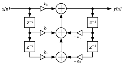
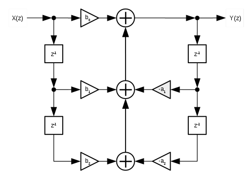
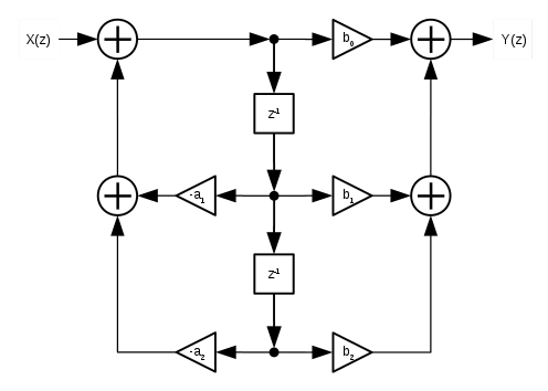
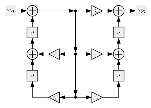
Direct Form I is characterized by having a total four unit delays present within it's architecture, with two coefficients (a1 and a2) arranged as to control negative coefficient gain (thus inverting the corresponding signal), and the remaining three (b0 to b2) controlling positive coefficient gain, with all feedback terms summed (added) together in a simple linear fashion;
Calculus:

Flow diagram:
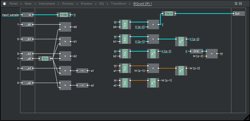
Implementation:
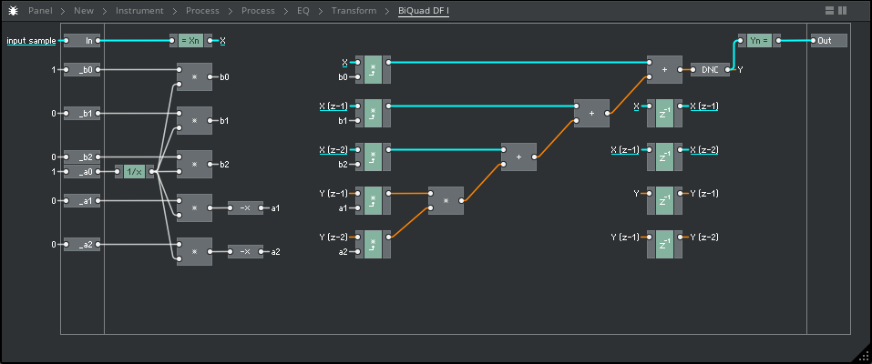
-
Blue cable = positive coeffiecient audio path
-
Red cable = negative ceofficient audio path
-
Grey cable = parameter value
Pseudo-code:
{
    X = input sample;

    _b0 = 1;
    _b1 = 0;
    _b2 = 0;
    _a0 = 1;
    _a1 = 0;
    _a2 = 0;

    a0 = (1 / a0_);

    a1 = (-1 * (a1_ * a0));
    a2 = (-1 * (a2_ * a0));

    b0 = (b0_ * a0);
    b1 = (b1_ * a0);
    b2 = (b2_ * a0);

    Y = ((X * b0) + (X(z-1) * b1) + (X(z-2) * b2) + (Y(z-1) * a1) + (Y(z-2) * a2));

    X(z-2) = X(z-1);
    X(z-1) = X;

    Y(z-2) = Y(z-1);
    Y(z-1) = Y;

    output sample = Y;
}
Notes:
DFI utlizes a total of four samples of delay ("z-1"). This (comparatively) higher number of unit delays present in the DFI structure make this arrangement relatively unstable when modulating the parameters while simultaneously passing audio, resulting in loud (and potentially damaging) clicks and pops in the resulting audio. In our test workbench (running as a VST3 effect in Reaper), even just moderate sweeps of the filter frequency control can incur signal overloads significant enough to trigger the in-built "channel auto-mute" safety feature, which avoids sending potentially damaging signals to the audio playback device and speakers.
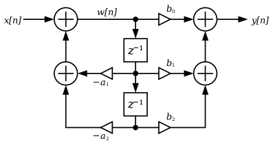
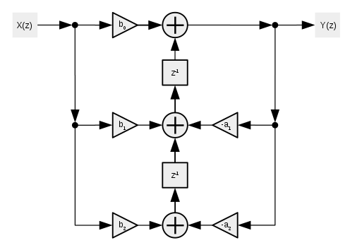
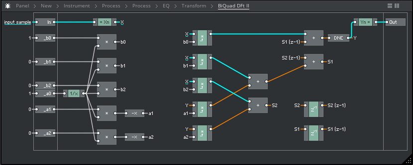
Direct Form II (also known as the "canonical" form, at least of the two discussed thus far) uses the same arrangement of coefficents, but only two unit delays - it also has what may be viewed as a "second" feedback path, here denoted as W(n);
Calculus:


Flow diagram:
Implementation:
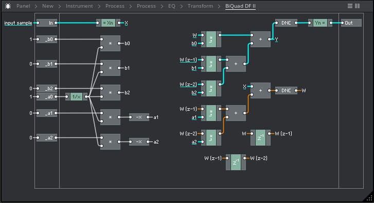
Pseudo-code:
{

    X = input sample;

    _b0 = 1;
    _b1 = 0;
    _b2 = 0;
    _a0 = 1;
    _a1 = 0;
    _a2 = 0;

    a0 = (1 / a0_);

    a1 = (-1 * (a1_ * a0));
    a2 = (-1 * (a2_ * a0));

    b0 = (b0_ * a0);
    b1 = (b1_ * a0);
    b2 = (b2_ * a0);

    W = (X + ((W(z-1) * a1) + (W(z-2) * a2)));
    Y = ((W * b0) + (W(z-1) * b1) + (W(z-2) * b2));

    W(z-2) = W(z-1);
    W(z-1) = W;

    output sample = Y;

}
Notes:
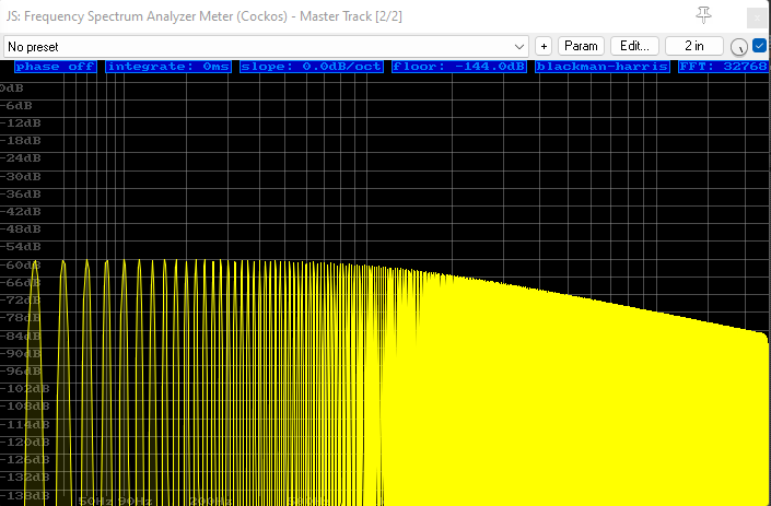
DFII, using less unit delays in it's architecture, produces much less significant artefacts during parameter modulation; in all but the most extreme cases, the output remains relatively benign. However, this structure is far more prone to "round-off" errors due to a narrowing computational precision in certain parts of the feedback network; this can manifest as a kind of "quantization noise" - much like un-dithered fixed-point audio - creeping well into the audible range, and in some cases enveloping low-amplitudinal parts of the input signal. This can be particularly extenuated by very large boosts of a tight "bell" shape in the lowest bass frequencies, causing strong quantization-error noise to permeate the upper-mid and treble ranges of the signal (image below).
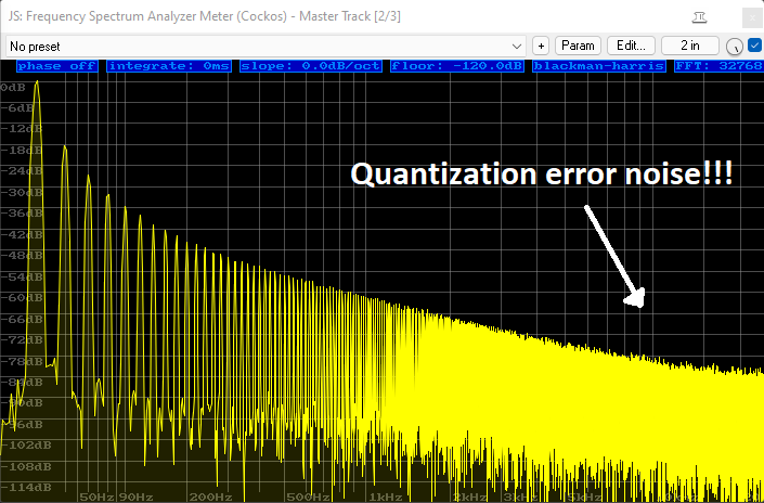
*(Shown above: +30dB boost at 20hz with Bandwidth of 1.0 using DFII, on a 20hz Sawtooth waveform)
For the "transposed" forms, all terms are inverted (signal flow reversed, summing points become split points, and multpiliers swap positions), creating the same output transfer function for the same number of components but in a somewhat "mirrored" directional flow of our input signal, resulting in our coefficient multiplications occuring before the unit delays;
Flow diagram:
Implementation:
Pseudo-code:
{

    X = input sample;

    _b0 = 1;
    _b1 = 0;
    _b2 = 0;
    _a0 = 1;
    _a1 = 0;
    _a2 = 0;

    a0 = (1 / a0_);

    a1 = (-1 * (a1_ * a0));
    a2 = (-1 * (a2_ * a0));

    b0 = (b0_ * a0);
    b1 = (b1_ * a0);
    b2 = (b2_ * a0);

    W = (X + W(z-2));
    Y = ((W * b0) + X(z-2));

    X(z-2) = ((W * b1) + X(z-1));
    X(z-1) = (W * b2);

    W(z-2) = ((W * a1) + W(z-1));
    W(z-1) = (W * a2);

    output sample = Y;

}
Notes:
The transposed Direct Form I ("DFI(t)") utilizes the four unit-delays of it's predecessor, meaning a higher memory footprint, while it also incurs the exact same "round-off error" and quantization noise as the original DFII structure. This is a dangerous combination for real-world audio use-cases, such as a mixing scenario.
So far, we've encountered one transformation resulting in zipper noise, one resulting in quantization noise, and one resulting in both.
This may seem discouraging, but we still have one final arrangement to try.
Direct Form II transposed only requires the two unit delays (like it's non-transposed counterpart), as opposed to the four of the Direct Form I (both counterparts), and likewise features it's multiplication coefficients happening before the unit delays occur;
Calculus:


Flow diagram:
Implementation:
Pseudo-code:
{

    X = input sample;

    _b0 = 1;
    _b1 = 0;
    _b2 = 0;
    _a0 = 1;
    _a1 = 0;
    _a2 = 0;

    a0 = (1 / a0_);

    a1 = (-1 * (a1_ * a0));
    a2 = (-1 * (a2_ * a0));

    b0 = (b0_ * a0);
    b1 = (b1_ * a0);
    b2 = (b2_ * a0);

    Y = ((X * b0) + (X(z-2)));

    X(z-2) = ((X * b1) + (X(z-1)) + (Y * a1));
    X(z-1) = ((X * b2) + (Y * a2));

    output sample = Y;

}
Notes:
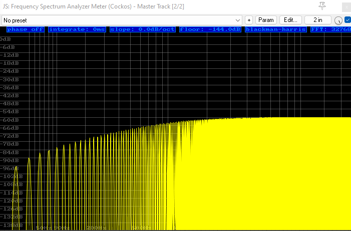
The Transposed Direct Form II, similarly to it's predecessor, uses only two unit-delays, making it much more amenable to audio-rate modulation; meanwhile, this form also successfully manages to avoid the higher "round-off" error and quantization noise of it's predecessor (and the DFI(t) structure).
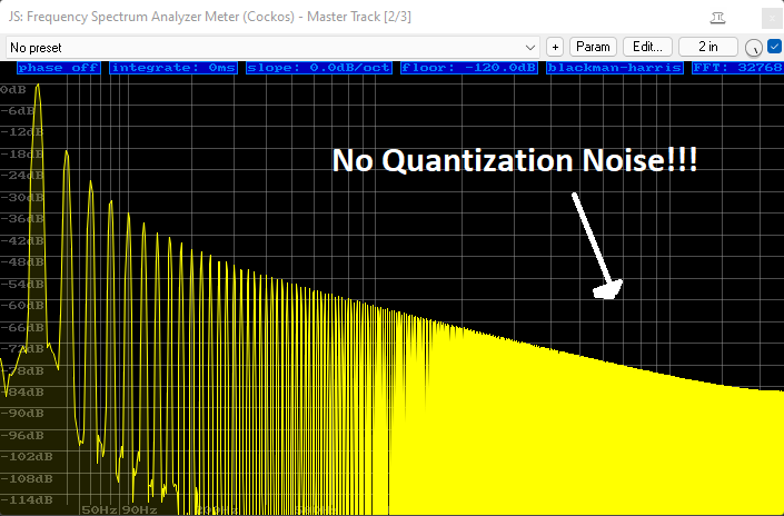
*(Shown above: +30dB boost at 20hz with Bandwidth of 1.0 using DFII(t), on a 20hz Sawtooth waveform)
As depicted in the above diagrams, the Direct Form I ("DFI") and II ("DFII") utlize a chain of single-sample unit delays in a feedback arrangement, with the coefficients a1 through to b2 controlling the gain at various points in the feedback network (in the case of DFII, actually two feedback networks).
The two "transposed" forms provide us the same output characteristics for the same number of components, but arranged in inverse terms as compared with the non-transposed forms; summing points become split points, gain multpiliers swap positions within the network, and the entire signal flow is reversed (our images are also flipped around to keep the input and output directions visually aligned with the previous structures).
This transposition places our coefficient multipliers before our unit delays, instead of after them.
I have seen some texts which provide several insights into what this change means with regards to our system stability and performance; one particularly intriguing which suggests that the transposed arrangements cause the unit delays (assumedly at their concurrent point of summation) act as a kind of smoother between changed values - perhaps very much like a single-pole low-pass filter? Another consideration might be the precision of our unit delays - let us imagine, for a moment, that our unit delays were operating at a lowly 16-bit fixed point arithmetic, causing truncation of the lowest bit ("least significant bit") of the audio data that we feed it. If we were to pipe our audio into our low-precision unit delay with a very low gain value (for example, we multiply by 0.0625 on the way in), and then compensate with a corresponding gain boost on the way out, we will have lost several bits of the "least significant part" of our audio to the low-precision unit delay. By contrast, if we were instead to pipe our audio into the unit delay at unity gain and then simply scale it to the appropriate level afterward, this gain scaling (coming after the unit-delay's truncation happens) does not affect our audio precision at all; any loss of "least significant" data going into the unit-delay has already happened before this scaling occurs.
Furthermore, we might want to consider how our coefficient calculations are being applied to the input signal "across time", on a sample-by-sample basis. This is where the relationship order of gain multiplier and unit delay becomes very important; if we consider that a single parameter, such as our "Q" control (adjusting our filter's bandwidth) is in fact updating several of our coefficient multipliers "simultaneously" by itself, then at what point in time do these various coefficient updates get applied to our audio stream?
As a slight abstraction, we can imagine that both "b2" and "a1" gain coefficients are updated simultaneously by our "Q" parameter on the GUI. Perhaps, one is the perfect inverse of the other;
when "b2 = 1, a1= -1",
just as when "a1 = -0.5, b2 = 0.5",
...and so on.
They are moving in perfectly complementary values at all times, instantaneously. So then what's the issue?
Well, what about our unit delays? Where are they placed within the path to to our audio stream? We can see that we have some instances in our various transformation types in which our gain multipliers are placed before the unit delays, and some structures which place the gain multipliers after the unit delays.
We can easily see that in the latter case, our gain calcuations are being applied instantaneously - that is, none of the calculation results are going through any unit delays. However, with the former, we see our gain calculations are infact "spread across time" by the various steps of unit delays in their paths.
So, what happens in either case when we update our "Q" parameter from the GUI, when b2 and a2 should travel in a perfectly complimentary fashion? Do they still converge upon complimentary numbers at the exact same time, considered on a sample-by-sample basis, with all these unit delays in their respective paths?
What if b2 moves and is applied via a single unit delay, while a1 takes an additional unit delay in it's path? Their respective numbers will no longer correspond in their intended fashion - b2 might move from, say, 1.0 to it's final value of 0.5, while a1 does both operations a single sample later, meaning that for the period of a single sample, our coefficients no longer converge upon the previously-specified algorithm's intended output values.
Thus, the levels of positive- and negative- gain within our structure may become completely unpredictable when modulated in real-time, causing completely unpredictable (and dangerously explosive) sonic results. This is clearly to be avoided at all costs in any real-world listening environment, which renders it rather useless for an audio application...!
This concept occured to the writer when considering whether applying smoothers to the coefficients b0 through a2 themeselves might combat some of the real-time modulation issues previously encountered. However, simply following the logic above, this idea would almost certainly make any of the transform structure completely unstable, causing more damage than good.
We can therefore conclude; It seems there are some quite terminal arguements for avoiding transformation structures that do not apply their gain coefficients simultaneously upon the audio path.
Of course, our circuit is much more complicated than this, especially as the number of poles (and zeros) grows - but these outlined concepts might at least help us gain some bearings on why these real-time performance differences arise between supposedly equal circuits.
Now, if we compare our results side by side, the results are interesting;
- DFI = four delay units (unstable modulation and higher footprint), higher precision (less quantization noise)
- DFII = two delay units (stable modulation and lower footprint), lower precision (more quantization noise)
- DFI(t) = four delay units (unstable modulation and higher footprint), lower precision (more quantization noise)
- DFII(t) = two delay units (stable modulation and lower footprint), higher precision (less quantization noise)
(images to follow)
As we can observe from the above comparison, our DFII(t) structure is the most favourable in all cases - it has only two delay units, meaning it is more stable under modulation, favourably comparable to the DFII structure; it also produces less quantization noise, comparable to the DFI structure in this regard. The lower unit delay count also produces a lower memory footprint in realtime use.
Our DFI(t) structure performs the most poorly in our highlighted cases - the quantization round-off error compares unfavourably to the DFII structure; while the four delay units contribute to heavy and unpredictable click/pop "zipper" noise underparameter modulation and also a higher memory footprint.
For a plugin designed for real audio mixing use cases, it's good practice to apply an appropriate amount of smoothing to all ranged parameters, in most cases. For now, smoothing has intentionally not been applied to the plugin's parameters, as this allows us to observe the differences between the four tranforms with respect to audio-rate modulation, one of the key issues with this entire filter design.
A parameter smoother may be applied in a future revision. However, during testing so far, it has been observed that a smoothed parameter, derived from a clock source that is likely asynchronous to the audio buffer clock, generates an unusual notch-like filter effect on the resulting audio spectrum whilst said parameter is under modulation; the deterministic frequency of this "notch-like" effect is seemingly related in periodicity to the parameter smoother's clock speed. Increasing precision to Doubles also seemingly eradicates the "notch-like periodicity" that our parameter smoother incurrs on the waveform to imperceptible levels.
Likewise, the quantization noise created by the feedback network's computational round-off errors can be seemingly entirely negated by increasing processing precision from Floats to Doubles; the resulting noise floor falls not only well below the audible threshold, but also below the reach of abilities of our testing software.
However, out of sight and out of mind does not mean out the window; we are able to produce several very pronounced audible artefacts in three of the four structures when processing in Floats (commonly deemed to be a beyond acceptable processing precision for audio purposes, to be debated elsewhere). Indeed only the Transposed Direct Form II manages favourably in all cases, and thus appears to be the prime candidate transformation for Biquad-based Equalizers in all audio application contexts at the time of writing. It stands to reason that these differences in quality shall also hold true (to some degree) for processing in Doubles, although we'd be extremely unlikely to encounter these differences when processing at that level of precision, seemingly well beyond the scope of measurement of our analysis tools - especially, and most critically, our ears.
- Nathan Hood (StoneyDSP), May 2022.
^ Credit: Smith, J.O. Introduction to Digital Filters with Audio Applications, http://ccrma.stanford.edu/~jos/filters/, online book, 2007 edition, accessed 02/06/2022.
^ Credit: Native Instruments for the Direct Form I code (taken from Reaktor 5's Core "Static Filter" library - go figure!) as well as the Core library unit delay, audio thread, and math modulation macros used here (I programmed the three other forms myself; both in Core and in C++).
^^ Reference: "Transformations" and "Calculus" images taken from: https://en.wikipedia.org/wiki/Digital_biquad_filter