Investigation of age-related changes in neuroblast populations using RNA velocity

Project overview

README file for a master project in Bioinformatics

• BINP52 - Master project - 60 ECTS
• Master programme in Bioinformatics
• Department of Biology, Faculty of Science, Lund University, Sweden

This work aimed to understand the aging signature on the neurogenesis process in the brain. For this purpose, three regions of mice brain, the Dentate Gyrus (DG), Subventricular zone (SVZ), and Olfactory Bulb (OB), in three age sample groups young (3 months), adults (14 months), and aged (24 months) were compared. This project provided an RNA velocity map of neurogenic niches of mice, together with substantial new knowledge about the biology of newly born neuroblasts and how they are affected by aging. Overall, our data advanced our understanding of the aging signature on the neurogenesis process in the brain.

People

• Student: Mostafa Torbati
• Supervisors: Henrik Ahlenius (henrik.ahlenius@med.lu.se) and Jonas Fritze (jonas.fritze@med.lu.se)
• Institute: Department of Clinical Sciences Lund, Division of Neurology, Lund Stem Cell Center, Lund University, Sweden
• Corresponding author: Mostafa Torbati

Hardware specifications

The following hardware was used:

• Apple MacBook Pro (Mid 2014, macOS Big Sur Version 11.7) used as a local computer.
• LUNARC's Aurora service HPC Desktop (High-performance computing), is used for preprocessing and visualizing the raw data.

Software versions

• Python 3.8.2
• JupyterLab 2.2.8
• 10x Genomics Cell Ranger v6.0
• Scanpy v1.7.2
• Velocyto v0.17.17
• ScVelo v0.2.4

Installation

On this project, we're working with large data and software such as Cell Ranger, which need High-performance computing (HPC) power. All the bioinformatics workflows for this project have been done on LUNARC Aurora service HPC Desktop ( the center for scientific and technical computing at Lund University). All the software is pre-installed on the LUNARC clusters so that users can access and load software packages based on the project's requirements. To efficiently management of the compute resources, we need to follow the SLURM job scheduler, which in simple words, is a bash script that loads all the necessary packages and sends it to the system backend. Here is an example of a bash script for submitting a job on Aurora:

#! /bin/bash
#SBATCH -A LSENS2018-3-3 # the ID of our Aurora project
#SBATCH -n 20 # how many processor cores to use
#SBATCH -N 1 # how many processors to use
#SBATCH -t 24:00:00 # kill the job after ths hh::mm::ss time
#SBATCH -J [JOB_NAME]# name of the job
#SBATCH -o [OUTPUT_report]%j.out # stdout log file
#SBATCH -e [ERROR_report]%j.err # stderr log file
#SBATCH -p dell # which partition to use
# load the necessary modules
module purge #remove all currently loaded modules 
module load [packages/software] #load packages
exit 0

The script is then submitted to the scheduler using the command:

sbatch my_script.sh

---

Flowchart

---

Data preparation with Cell Ranger workflow

Build a Custom Reference

For this project, we used transgenic mice in which Enhanced Green Fluorescent Protein (EGFP) is expressed under the control of the DCX promoter. As EGFP is not included in the pre-built reference genome, we first created a custom reference genome and added EGFP to an existing mouse reference.

The cellranger mkref command is used to build a custom reference for use with the Cell Ranger pipeline.

Prepare input files

• The following files are required to build the reference:
• FASTA file containing the genome sequences
• GTF file containing the gene annotation

get the FASTA file

wget ftp://ftp.ensembl.org/pub/release-102/fasta/mus_musculus//dna/Mus_musculus.GRCm38.dna.primary_assembly.fa.gz

get the GTF file

wget ftp://ftp.ensembl.org/pub/release-102/gtf/mus_musculus//Mus_musculus.GRCm38.102.chr.gtf.gz

filter the GTF file

GTF files can contain entries for non-polyA transcripts that overlap with protein-coding gene models.To remove these entries from the GTF, we need to use cellranger mkgtf nad add the filter argument --attribute=gene_biotype:protein_coding to the mkgtf command:

#! /bin/bash
#SBATCH -A LSENS2018-3-3 # the ID of our Aurora project
#SBATCH -n 20 # how many processor cores to use
#SBATCH -N 1 # how many processors to use
#SBATCH -t 24:00:00 # kill the job after ths hh::mm::ss time
#SBATCH -J filter_gtf_Mus # name of the job
#SBATCH -o filter_gtf_Mus%j.out # stdout log file
#SBATCH -e filter_gtf_Mus%j.err # stderr log file
#SBATCH -p dell # which partition to use
module purge
module load cellranger/6.0.0 \
cellranger mkgtf [PATH_TO_GTFfile]\
Mus_musculus.filtered_gtf.gtf \ #This will output the file Mus_musculus.filtered_gtf.gtf, which will be used in the cellranger mkref step.
--attribute=gene_biotype:protein_coding
exit 0

Setup the command for cellranger mkref

#! /bin/bash
#SBATCH -A LSENS2018-3-3 # the ID of our Aurora project
#SBATCH -n 20 # how many processor cores to use
#SBATCH -N 1 # how many processors to use
#SBATCH -t 24:00:00 # kill the job after ths hh::mm::ss time
#SBATCH -J mkref_Mus_musculus # name of the job
#SBATCH -o mkref_Mus_musculus%j.out # stdout log file
#SBATCH -e mkref_Mus_musculus%j.err # stderr log file
#SBATCH -p dell # which partition to use
module purge
module load cellranger/6.0.0
cellranger mkref --genome=Mus.musculus_genome \ #name of the custom reference folder
--fasta=[replace with the path of FASTA file containing the genome sequences] \
--genes=[replace with the path  of _Mus_musculus.filtered_gtf.gtf_ created in the previous step]
exit 0

Add a marker gene (EGFP) to the FASTA and GTF

get the EGFP gene sequence EGFP complete sequence

Edit the header of EGFP fasta file tp make it more informatice

>EGFP
TAGTTATTAATAGTAATCAATTACGGGGTCATTAGTTCATAGCCCATATATGGAGTTCCGCGTTACATAA
CTTACGGTAAATGGCCCGCCTGGCTGACCGCCCAACGACCCCCGCCCATTGACGTCAATAATGACGTATG
TTCCCATAGTAACGCCAATAGGGACTTTCCATTGACGTCAATGGGTGGAGTATTTACGGTAAACTGCCCA
CTTGGCAGTACATCAAGTGTATCATATGCCAAGTACGCCCCCTATTGACGTCAATGACGGTAAATGGCCC
GCCTGGCATTATGCCCAGTACATGACCTTATGGGACTTTCCTACTTGGCAGTACATCTACGTATTAGTCA
TCGCTATTACCATGGTGATGCGGTTTTGGCAGTACATCAATGGGCGTGGATAGCGGTTTGACTCACGGGG
ATTTCCAAGTCTCCACCCCATTGACGTCAATGGGAGTTTGTTTTGGCACCAAAATCAACGGGACTTTCCA
AAATGTCGTAACAACTCCGCCCCATTGACGCAAATGGGCGGTAGGCGTGTACGGTGGGAGGTCTATATAA
GCAGAGCTGGTTTAGTGAACCGTCAGATCCGCTAGCGCTACCGGACTCAGATCTCGAGCTCAAGCTTCGA
ATTCTGCAGTCGACGGTACCGCGGGCCCGGGATCCACCGGTCGCCACCATGGTGAGCAAGGGCGAGGAGC
TGTTCACCGGGGTGGTGCCCATCCTGGTCGAGCTGGACGGCGACGTAAACGGCCACAAGTTCAGCGTGTC

We need to count the number of bases in the sequence:

cat EGFP.fa | grep -v "^>" | tr -d "\n" | wc -c

The results of this command shows there are 4733 bases. This is important to know for the creating custom GTF for EGFP.

Now to make a custom GTF for EGFP with the following command:

Note: we need to insert the tabs that separate the 9 columns of information required for GTF.

echo -e 'EGFP\tunknown\texon\t1\t4733\t.\t+\t.\tgene_id "EGFP"; transcript_id "EGFP"; gene_name "EGFP"; gene_biotype "protein_coding";' > EGFP.gtf

This is what the EGFP.gtf file looks like with the cat EGFP.gtf command:

EGFP	unknown	exon	1	4733	.	+	.	gene_id "EGFP"; transcript_id "EGFP"; gene_name "EGFP"; gene_biotype "protein_coding";

Next, add the EGFP.fa to the end of the M. musculus genome FASTA. But first, make a copy so that the original is unchanged.

cp Mus_musculus.filtered_gtf.gtf Mus_musculus.filtered_gtf_EGFP.gtf

Now append EGFP.fa to Mus_musculus.filtered_gtf_EGFP.gtf as following:

cat EGFP.fa >> Mus_musculus.filtered_gtf_EGFP.gtf

Use cellranger mkref command to create custom reference directory with EGFP added

Now use the genome_Mus_musculus_EGFP.fa and Mus_musculus.filtered_gtf_EGFP.gtf files as inputs to the cellranger mkref pipeline:

#! /bin/bash
#SBATCH -A LSENS2018-3-3 # the ID of our Aurora project
#SBATCH -n 20 # how many processor cores to use
#SBATCH -N 1 # how many processors to use
#SBATCH -t 24:00:00 # kill the job after ths hh::mm::ss time
#SBATCH -J addGFP_Mus_musculus # name of the job
#SBATCH -o addGFP_Mus_musculus%j.out # stdout log file
#SBATCH -e addGFP_Mus_musculus%j.err # stderr log file
#SBATCH -p dell # which partition to use
module purge
module load cellranger/6.0.0
cellranger mkref --genome=Mus.musculus_genome_EGFP \
--fasta=genome_Mus_musculus_EGFP.fa \
-genes=Mus_musculus.filtered_gtf_EGFP.gtf
exit 0

This outputs a custom reference directory called Mus.musculus_genome_EGFP/.

Converting RAW data to FASTQ files

Raw base call (BCL) was provided for this project from Illumina sequencers. 10X Genomics describes several scenarios about how to design the workflow of the experiments. Based on each scenario, we need to follow a specific CellRanger pipeline. Here is the schematic description of our scenario:

One sample, one GEM well, multiple flow cells

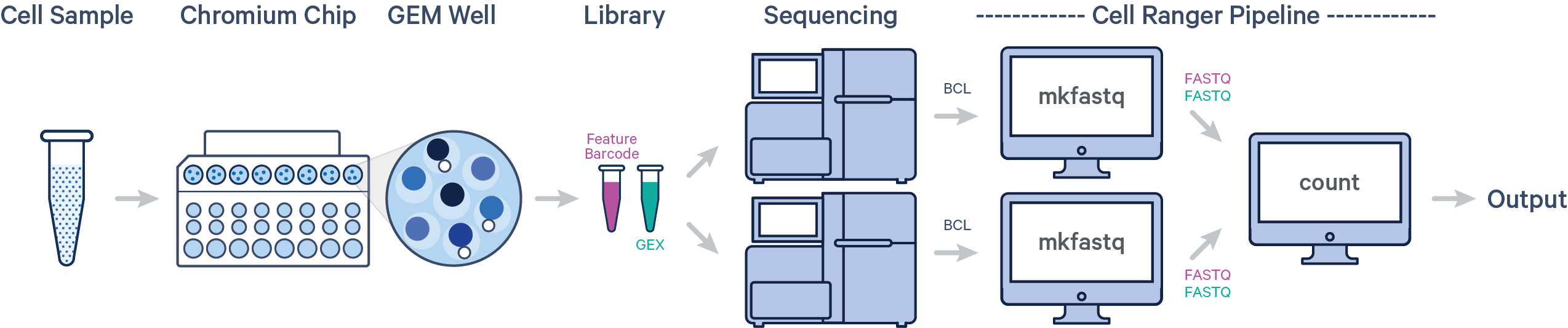
In this example, one sample is processed through one GEM well, resulting in one library which is sequenced across multiple flow cells. This workflow is commonly performed to increase sequencing depth.

CellRanger pipeline based on this workflow:

1. Convert BCL files obtained from Illumina sequencer to FASTQ files usisng cellranger mkfastq
2. cellranger count that takes FASTQ files from cellranger mkfastq and performs alignment, filtering, barcode counting, and UMI counting. It uses the Chromium cellular barcodes to generate feature-barcode matrices, determine clusters, and perform gene expression analysis. Implementing this pipeline allows all reads to be combined in a single instance.

Run cellranger mkfastq for the fisrt sequencing run

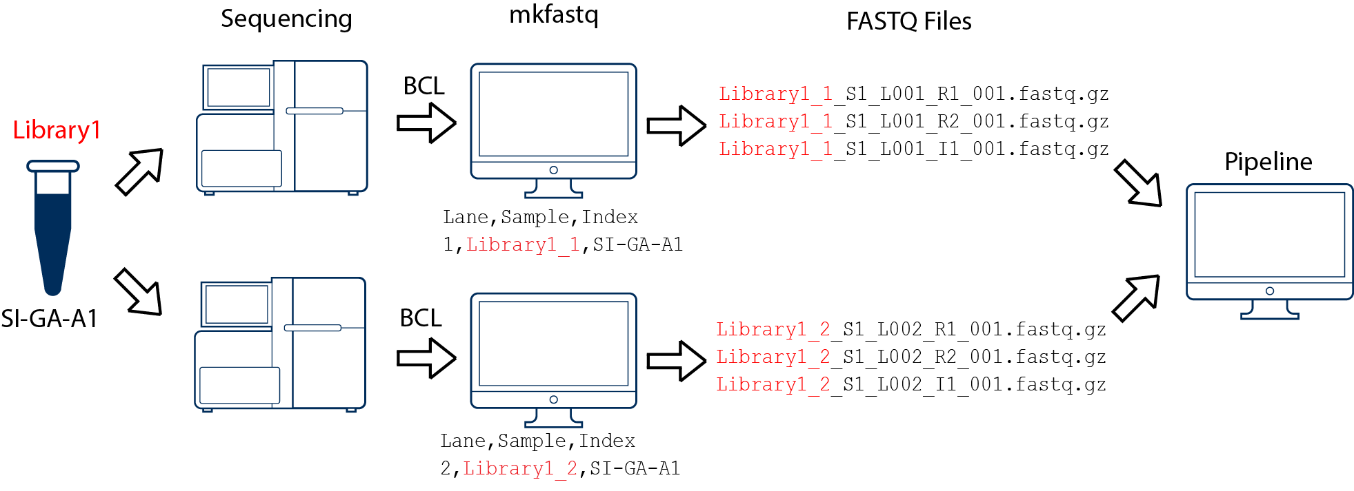
In our case, we have one 10x Genomics library sequenced on two flow cells. Note that after running cellranger mkfastq, we run a single instance of the cellranger pipeline on all the FASTQ files generated:

Run the command on LUNARC:

#! /bin/bash
#SBATCH -A LSENS2018-3-3
#SBATCH -n 20
#SBATCH -N 1
#SBATCH -t 24:00:00
#SBATCH -J mkfasta
#SBATCH -o mkfastq_1stRun%j.out
#SBATCH -e mkfastq_1stRun%j.err
#SBATCH -p dell
module --force purge
module load SoftwareTree/Haswell
module load GCCcore/6.3.0
module load bcl2fastq/2.19.1
module load CellRanger/7.0.0
cellranger mkfastq --id=mkfastq_1stRun \ #output folder for the 1st run
--run=181023_NB502004_0035_AHWGGFBGX5 \ #folder containing BCL files from 1st sequencing run
--csv=Library_concentration.csv #Path to a simple CSV with lane, sample, and index columns, generated by sequencer software which describe the way to demultiplex the flow cell.
exit 0

Running this code successfully generates a directory containing the sample folders (it'smkfastq_1stRun in our case) would be named according to the flow cell ID.

Run cellranger mkfastq for the second sequencing run

#! /bin/bash
#SBATCH -A LSENS2018-3-3
#SBATCH -n 20
#SBATCH -N 1
#SBATCH -t 24:00:00
#SBATCH -J mkfasta
#SBATCH -o mkfastq_2ndRun%j.out
#SBATCH -e mkfastq_2ndRun%j.err
#SBATCH -p dell
module --force purge
module load SoftwareTree/Haswell
module load GCCcore/6.3.0
module load bcl2fastq/2.19.1
module load CellRanger/7.0.0
cellranger mkfastq --id=mkfastq_2ndRun \ #output folder for the 2nd run
--run=181024_NB502004_0036_AHW7FCBGX5 \ #folder containing BCL files from 2nd sequencing run
--csv=Library_concentration.csv ##Path to a simple CSV with lane, sample, and index columns, generated by sequencer software which describe the way to demultiplex the flow cell.
exit 0

Running this code successfully generates a directory containing the sample folders (it'smkfastq_2ndRun in our case) would be named according to the flow cell ID.

By running cellranger mkfastq on the Illumina BCL we ended up with two folders containing FASTQ files for each sequencing run which will be used in the next step.

Cell Ranger count pipeline

The count pipeline is the next step after mkfastq. In this step FASTQ files from two sequencing libraries and generates a count matrix, which is a table of the number of times each gene was detected in each cell. This matrix is then used as input for downstream analysis, such as identifying differentially expressed genes or clustering cells into groups. The pipeline does this by using a series of steps, including quality control, alignment, and quantification of reads.

#! /bin/bash
#SBATCH -A LSENS2018-3-3
#SBATCH -n 20
#SBATCH -N 1
#SBATCH -t 24:00:00
#SBATCH -J Run_DG3_count
#SBATCH -o DG3count%j.out
#SBATCH -e DG3count%j.err
#SBATCH -p dell
module --force purge
module load SoftwareTree/Haswell
module load cellranger/6.0.0
cellranger count --id=DG3_count \ #output folder
--fastqs=/mkfastq_1stRun/outs/fastq_path/Chromium_20180912,/mkfastq_2ndRun/outs/fastq_path/Chromium_20180912 \ #two comma-separated of FASTQ paths
--sample=DG3 \
--transcriptome=custom_ref_gene/Mus.musculus_genome_EGFP
exit 0

--fastqs in the cellranger countpipeline, we can add multiple comma-separated paths of FASTQ files for this argument. Doing this will treat all reads from the library, across flow cells, as one sample. This approach is essential when we have the same library sequenced on multiple flow cells.

--sampleargument takes the sample name as specified in the sample sheet supplied to cellranger mkfastq.

--transcriptome import the the custom reference genome that we created with the cellranger mkref.

For this project, we have nine samples of three age groups from 3 neurogenic niches of mice brains, Dentate Gyrus (DG), Subventricular Zone (SVZ), and Olfactory Bulb (OB). We must repeat the cellranger count pipeline for each region and age group.

cellranger count generates multiple outputs in different formats which can be used for many downstream analysis.

Velocyto Run on 10X Chromium samples

We need to combine spliced and unspliced RNA-seq data for the velocity analysis. For this purpose, we use the Velocyto command line tool. Velocyto provides tools for different technologies. We use run10xas our samples are generated through 10X Chromium technology.

Example bash script on LUNARC

#!/bin/sh
#SBATCH -n 20
#SBATCH -N 1
#SBATCH -t 20:00:00
#SBATCH -A lsens2018-3-3
#SBATCH -p dell
#SBATCH -J velocyto
#SBATCH -o DG3_velocyto.%j.out
#SBATCH -e DG3_velocyto.%j.err
module purge
module load GCC/10.2.0
module load velocyto/0.17.17
module load SAMtools/1.12
repeats="mm10_rmsk.gtf"
transcriptome="EGFP.gtf"
cellranger_output="/cellranger_count/DG3/DG3_count"
velocyto run10x -m $repeats \
                $cellranger_output \
                $transcriptome
exit 0

We need to run this code for each of our nine samples. This pipeline will generate a folder in the cellranger count output folder, which contain a loom file for spliced and unspliced regions.

Scanpy and ScVelo

The rest of the analysis performs on Jupyter Notebook, and the prepared data is implemented on the Scanpy package for Pre-processing and ScVelo for RNA velocity.

References

10x Genomics Cell Ranger v6.0

Wolf, F., Angerer, P. & Theis, F. SCANPY: large-scale single-cell gene expression data analysis. Genome Biol 19, 15 (2018).

La Manno et al. (2018), RNA velocity of single cells, Nature.

Bergen et al. (2020), Generalizing RNA velocity to transient cell states through dynamical modeling, Nature Biotech.

Bergen et al. (2021), RNA velocity - current challenges and future perspectives, Molecular Systems Biology.

Copyright

Copyright © Mostafa Torbati, Department of Clinical Sciences, Division of Neurology, Lund Stem Cell Center, Lund University, Sweden