Databases

Below are my study notes from an excellent lecture on Database Systems (Part I: Theory, Part II: Design) by Prof. Trummer at Cornell. I've made these notes to further my understanding of database theory and the inner-workings of database management systems. A companion book for this lecture is: Database Management Systems by Johannes Gehrke and Raghu Ramakrishnan.

Databases

Introduction To Database Systems

Database Management Systems (DBMS)

On the surface it seems simple enough, an application queries a database which then returns some data. But between the data and the interface of the DBMS lies a stack of processors and managers that ensure queries and data are handled in specific ways.

Structured Query Language (SQL)

To interface with the DBMS we must use SQL to issue queries. These queries, or commands, can be distinguished by the types of tasks they perform within the DBMS:

Data Control Language (DCL) -> exists to assign access rights to data
Transaction Control Language (TCL) -> groups SQL commands as transactions
Data Manipulation Language (DML) -> insert, manipulate, and retrieve data
Data Definition Language (DDL) -> defines what is admissible data within set constraints

# fully specified
insert into <table> values (<val-list>);
# partially specified
insert into <table> (<col-list>) values (<val-list>);

Data Definition Language (DDL)

With DDL we define a database schema that describes the content we can have in our database. A schema in a relational database consists as a collection of two-dimensional arrays of information labeled with columns and each column is associated with a datatype. The data that is accepted by the scheme is defined by constraints which either link single relations or multiple relations.

id	name	surname	age	license-driving
1	mark	lasperre	42	1234-4321-1234-1234
2	tom	gershwin	69	4321-1234-1234-1234
3	travis	nakumi	34	1234-1234-1234-4321

Schema Definition in SQL

In SQL specifically, we don't talk about relations, we talk about tables. There are fine differences between relations in the Relational Data Model and tables in SQL but superficially they can be used to mean the same thing.

CREATE TABLE Students(Sid int, Sname text, Gpa real);
CREATE TABLE Enrollment(Sid int, Cid int);
CREATE TABLE Courses(Cid int, Cname text);

CREATE TABLE <table> (<table-def>)
# <table> is the table name
# <table-def> is comme-separated column definitions
# <col-name><col-type> is the form for definitions

Integrity Constraints

Above we have created three tables. Each column has a name, a key if you will, and a datatype associated with that column. The datatype is what is called an Integrity Constraint, as the DBMS enforces what types of data are permissible for each column ensuring the integrity of the model.

Primary Key Constraints

A primary key constraint refers to a single table in the schema which contains a column of keys of which no two rows are allowed to have the same value. The primary key is in effect the ID for that given row in relation to the rest of the schema.

It is possible to alter the existing tables we created by issuing the following command:

ALTER TABLE <table> ADD Primary Key (<key-cols>);
# <table> is the table name
# <key-cols> is the list of column names

ALTER TABLE Students ADD PRIMARY KEY(Sid);
ALTER TABLE Enrollment ADD PRIMARY KEY(Sid, Cid);
ALTER TABLE Courses ADD PRIMARY KEY(Cid);

Every table can have only one Primary Key, but you can have multiple columns in your Primary Key, which we call a Composite Primary Key. This Composite Primary Key exists in what is commonly called a Link, Join, or Junction Table. This Junction Table contains only Foreign Keys in order to facilitate a many-to-many relationship.

In the case of our example above, the Enrollment table has a Student ID and a Course ID, and neither are unique on their own, but combined they represent a unique combination that becomes our Composite Primary Key. So the Student ID in the Students table links to the Enrollment table which then is paired with a Course ID which links the Enrollment table to the Courses table.

Students Table	Enrollment Table	Courses Table
[Sid , Sname, Gpa]	[Sid, Cid]	[Cid, Cname]
Pkey: Sid	Pkey: Sid, Cid	Pkey: Cid

Foreign Key Constraint

A Foreign Key links two tables by identifying a group of columns in one table and mapping those columns to the primary key of another table, those Foreign Key column values must appear as Primary Keys in the related table and is how we map each row from the first table to the second table.

ALTER TABLE <table-1> ADD Foreign Key (<fkey-cols>)
REFERENCES <table-2> (<pkey-cols>);
# <table-1> is the table that contains foreign key columns <fkey-cols>
# <table-2> is the table that contains primary key columns <pkey-cols>

Here we create a link from the Student ID in the Enrollment table to the Student ID in the Students table and the Course ID in the Enrollment table to the Course ID in the Courses table. In both instances we tell the current table we are referencing a Primary Key from another table. In the land of tables, if tables were countries, this Primary Key originates from a foreign table, so it is a Foreign Key.

ALTER TABLE Enrollment ADD FOREIGN KEY(Sid) REFERENCES Students(Sid);
ALTER TABLE Enrollment ADD FOREIGN KEY(Cid) REFERENCES Courses(Cid);

Introduction To SQL

Data Manipulation Language (DML)

Commands which are responsible for allowing CRUD operations to take place in the database.

Insert
Delete
Update
Analyze

Inserting Data

We can insert fully specified or partially specified data into rows. Fully specified means we specify the value for each column in the table, hence we fully specify what we want to be inserted. Partially specified, means we only target a specific column or subset of columns, and the DBMS fill the remaining columns automatically with NULL unless there is an integrity constraint which does not allow for NULL.

Deleting Data

Deleting data from tables can be achieved with DELETE FROM <table> WHERE <condition>. For instance, Pageturners has been told Jimmy Droptables wasn't an author on Database Guru.

# We can delete him from the join table called authors.
delete from authors where writerid = 6;
delete from writers where writerid = 6;

Updating Data

Updating data, much like delete, has a simple syntax: UPDATE <table> SET <col> = <val> WHERE <condition>. Pageturners has been told Jane Droptables is actually Jane Hadersville!

# Let's update her name before someone notices.
update writers set last_name = 'Hadersville' WHERE writerid = 7;

Simple SQL Data Analysis

An SQL query is a new relationship that has to be generated by the DBMS. We describe our desired output as a query and the system has to figure out how to display that output. Most SQL queries consist of three parts. SELECT which describes column relation, FROM which describes source relations, and WHERE which defines conditions which need to be satisfied before we can receive a result. The majority of syntax needed for a SQL query can be reduced to the following: select <col> from <table-1> join <table-2> on <join-condition> where <where-condition>

# Let's see if we can perform a query on our pageturnersdb to return all work by Marcus Aurelius
SELECT books.booktitle
FROM books
JOIN authors ON (books.bookid = authors.bookid)
JOIN writers ON (authors.writerid = writers.writerid)
WHERE writers.writerid = 2;
# You'll notice because the data is related, it's possible to retrieve 
# the queries intended answer in more than one way.
SELECT books.booktitle
FROM books
JOIN authors ON (books.bookid = authors.bookid)
JOIN writers ON (authors.writerid = writers.writerid)
WHERE (writers.first_name) = 'Marcus';

Simplification by Alias

To save ourselves some time while writing queries, it is possible to alias table names in the following manner.

SELECT b.booktitle
FROM books b
JOIN authors a ON (b.bookid = a.bookid)
JOIN writers w ON (a.writerid = w.writerid)
WHERE (w.first_name) = 'Marcus';

Predicate Statements

A predicate is not a conditional. A conditional statement allows for branching logic whereas a predicate is a question that results in either boolean true or boolean false. SQL support many types of predicates that return a boolean value when they resolve.

Inequality (>, >=): books.bookrating > 80
Not Equal (<>): books.booktitle <> 'Life of Pi'
Exists in list (IN): booktitle IN ('list_item', 'list_item_2')
Regular Expression: (LIKE): WHERE booktitle LIKE 'L__%'

Composite Predicates

Logical conjunction: AND
Logical disjunction: OR
Negation: NOT

Select Clauses

Wildcard selection of multiple columns: *
Select all columns from a table: <table>.*
Expressions in the select clause: SELECT 3 * (<col1> + <col2>)
Alias assignment for output columns: SELECT bookname as booktitle

Join Syntax

Standard join: <table1> JOIN <table2> ON (<table1>.<col> = <table2>.<col>)
Abreviated join: <table1> JOIN <table2> USING (<col>)
Natural join: automatically join columns with the same name: <table1> NATURAL JOIN <table2>
Terse form of a Standard join: FROM <table1>, <table2> WHERE <join-condition>

Distinct

Eliminate duplicates using SELECT DISTINCT

Aggregation

Numerical expressions: SUM, AVG, MIN, MAX
Count rows in result: COUNT(*)
Count result row in column: COUNT(<col>)
Count distinct values in column: COUNT(DISTINCT <col>)
Aggregating multiple columns: GROUP BY <col-list>

example: let's count the the remaining rows with COUNT(*)

SELECT COUNT(*)
FROM books
    JOIN Authors ON (books.bookid = authors.bookid)
    JOIN Writers ON (authors.writerid = writers.writerid)
WHERE books.booktitle = 'Life of Pi';

Group Predicates

WHERE applies to a single row
HAVING specifies grouped data

Ordering Syntax

We can use ORDER BY to arrange an <order-item-list>
The syntax is: <order-item>:<col> <direction>
The direction can be ASC ascending or DESC desending.
Is applied after grouping when using group-by queries.

More Advanced SQL Features

Unknown Values

In SQL, an unknown value is referred to as NULL, NULL is not ZERO, it is the absence of a value, or a value which holds no type. Because SQL uses Ternary (three-valued) logic, the outcome of a logical predicate can be either true, false or unknown (NULL). We check the outcome of an expression with = True, = False, and IS NULL.

Ternary Logic Examples with NULL.

SELECT 3 = NULL will result in NULL, not False
SELECT NULL = NULL will result in NULL, not True
SELECT NULL IS NULL will result in True
SELECT NULL IS NOT NULL will result in False
SELECT TRUE OR NULL will result in True
SELECT TRUE AND NULL will result in NULL

Joins with Unknowns

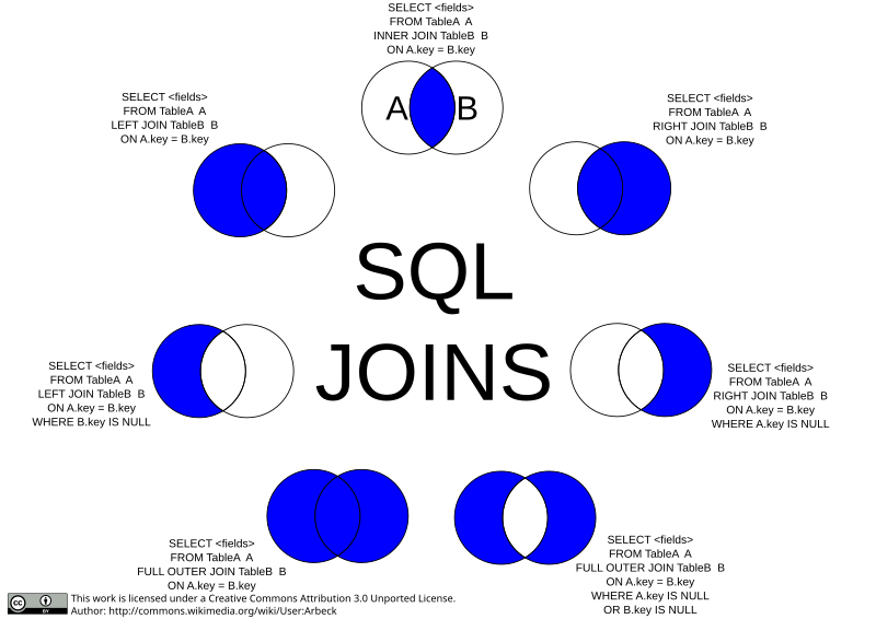
A standard join keeps only matching row pairs. It eliminates rows without matching rows in other tables. Sometimes we want to keep rows regardless, to achieve this we can perform an OUTER JOIN, this type of join will fill missing field data with NULL values in order to maintain partial rows.

<table1> LEFT OUTER JOIN <table2> ON ... - Keeps rows in left table
<table1> RIGHT OUTER JOIN <table2> ON ... - Keeps rows in right table
<table1> FULL OUTER JOIN <table2> ON ... - Keeps rows in both tables

example: We want to see the number of enrollments per student

SELECT studentname, COUNT(courseid)
FROM studenttable LEFT OUTER JOIN enrollmenttable
ON (studenttable.studentid = enrollmenttable.studentid)

In the above example, if a student does not have matching enrollment information the join operation will assing null values in the students courseid fields, and then those null values will not be counted when performing the query.

Set Operations

A powerful feature of SQL is the ability to combine queries, in effect creating composite queries. The easiest way to do this is to use Set Operations on compatible queries.

<query-1> UNION <query-2> - This eliminates duplicates
<query-1> UNION ALL <query-2> - This preserves duplicates
<query-1> INTERSECT <query-2> - This preserves similarities between query results
<query-1> EXCEPT <query-2> - This preserves differences between query results

All of the above Set Operations must be union-compatible, in other words they must have the same structure (number of columns, column names, etc.)

Query Nesting

With nesting we can use queries as part of other queries, for example we can say FROM <query> replacing the table, and as part of a condition in a WHERE clause, WHERE <query>. The smaller queries inside the larger query are called sub-queries. Formally, in the context of this relationship, a query is referred to as a containing query and a sub-query is referred to as a contained query. Sub-queries that can run independently, in other words that are not dependant on their containing query to produce a result (self-contained), are called Uncorrelated sub-queries. Correlated sub-queries can reference their containing queries.

Uncorrelated examples: Inner queries can run independently from their containing queries.

SELECT subquery.studentname FROM(SELECT studentname FROM studentstable) AS subquery;
SELECT studentname FROM studentstable WHERE gpa >= (SELECT MAX(gpa) FROM studentstable);

Correlated example: Inner queries are dependant on their containing queries.

SELECT s1.studentname FROM studentstable s1 WHERE s1.gpa >= ALL(SELECT s2.gpa FROM studentstable s2 WHERE s1.studentname = s2.studentname)

Multiple nested queries example: Queries nested in queries nested in queries.

SELECT course.coursename FROM coursestable course WHERE NOT EXISTS (SELECT * FROM studentstable student WHERE NOT EXISTS( SELECT * FROM enrollmenttable enrolled WHERE enrolled.courseid = course.courseid AND enrolled.studentid = student.studentid))

Sub-Queries in Conditionals

It is possible to use sub-queries in conditional statements that will resolve to a boolean value. For instance, we can check to see if a sub-query returns an empty result by issuing: EXISTS(<sub-query>), which will return TRUE if not empty. We can also check for a specific value in a sub-query: <value> IN (<sub-query>), which will resolve to TRUE if the value matches. It is also possible to check if a condition holds true for ALL rows: >= ALL(<sub-query>) or only some. ANY: >= ANY(<sub-query>)

Here we check for students where gpa is greater or equal to the gpa of all students, this will result in the query returning the maximum gpa. You can conceptualize this nested query as being two nested for-loops, although this is not what the Database System is actually doing to the data.

SELECT studentname FROM studentstable WHERE gpa >= (SELECT gpa FROM studentstable);

Data Storage

Data Storage Hardware

The Memory Hierarchy in Computer Science, refers to the relation between access speed and storage capacity. Usually, the higher the speed, the lower the capacity, and so this creates a triangle with very fast memory inside the CPU called registers at the top of the pyramid and slower magnetic tape backups at the bottom. It is also important to remember that storage is either volatile or non-volatile, meaning data will either disappear once power is cycled, or persist in a stable way between states. Data must move through this hierarchy up towards the processor, so the processor can access the stored information.

Registers -- Volatile
- Fastest Access
- Smallest Capacity
- Highest Cost
- Limited Function
CPU Cache -- Volatile
- L1 (fastest), L2 (faster), L3 (fast) Caches
- Near Instantaneous Access (~1 Nanosecond)
- Very High Bandwidth (Hundreds to Thousands of GB/s)
- Very Low Capacity (Tens of Kilobytes)
- Very Expensive (Hundreds of $/GB)
Main Memory -- Volatile
- Very Fast Access (~Tens of Nanoseconds)
- Low Capacity (Tens to Hundreds of Gigabytes)
- High Bandwidth (~GB/s)
- Expensive (Many $/GB)
Flash Memory -- Non-Volatile
- Fast Access (~1 Millisecond)
- High Capacity (Tens to Hundreds of Terabytes)
- Elevated Read Speed (500MB/s)
- Less Cheap ($0.25/GB)
Hard Disks -- Non-Volatile
- Slow Access (10s of Milliseconds)
- Moderate Capacity (Tens of Terabytes)
- Moderate Read Speed (~200MB/s)
- Cheap ($0.035/GB)
Tape Backups -- Non-Volatile
- Slow Access (10s of Seconds)
- Highest Capacity (Hundreds of Terabytes)
- Moderate Read Speed (~300MB/s)
- Very Cheap ($0.02/GB)

Relevance for DBMS

Databases management system design is influenced by the memory hierarchy. Capacity limits force data down the hierarchy and access speed, which becomes a bottleneck the lower we go down the hierarchy, is influenced by how the databases algorithms were created. Random access to data is 'expensive', in Computer Science terms this costliness is described with mathematical notation referred to as big-O notation, which describes "limiting behavior of a function when the argument tends towards a particular value".

When designing databases, we ideally want to optimize our system to minimize data movement, this can be achieved by reading data in larger chunks (pages) and keep related data closer together to make the access more efficient. Another consideration is volatility and the ability to recover from failure in the memory hierarchy.

Data Storage Formats

Tables as Files

We can store the information or meta-data for the Table Schema in a database catalogue, the content of tables are then stored as a collection of pages (files), with each page storing a few KB of data. They can store multiple rows but not entire tables. The size of these pages are chosen to maximize retrieval efficiency in relation to the storage medium.

From Files to Pages

How do we keep track of which pages store information for which tables? One possibility is to use doubly linked lists where each page contains pointers to next and prior pages, optionally we can have pages that are full and pages that are empty so we do not waste time trying to write to full pages. Another possibility is to create a directory of pointers to pages, where the directory header page makes reference to directory pages, which in turn reference data pages with meta-data.

From Pages to Slots

We need to be able to partition pages into sections that store different rows. To achieve this pages are divided into slots, and each slot stores one record (table row). Top refer to one specific row, we just need the pageID and slotID which both together become the recordID. There are multiple ways to device pages into slots dictated by the fixed-length vs variable length of records.

Fixed-Length Records

Data types like integers can be determined apriori due to the fixed quantity of bytes (4) needed to create one unit of said datatype. This means it is much easier to work with fixed-length data types, which can be uniformly partitioned into set sized records, as opposed to text strings, which are variable, and therefore not determinable a-priori. We must still keep track of how these slots are used (insertions), this is achieved with packed representation, or unpacked representation. Packed representation uses consecutive slots and only keeps track of number of slots used, whereas the unpacked method allows unused slots in-between used slots, but needs a bitmap to keep track of used slots. A potential issue with packed representation is that removing a slot (deletion) leaves a hole, which has to be filled, which effects the slotID, meaning we would have to update any external references.

Variable-Length Records

If we have data types that require a variable number of bytes in order to store an entry, the task of creating records becomes slightly more difficult. We can create a what is called an on-page directory concerned with used slots which stores a reference to the first byte and the length of slots. This allows us some flexibility to move around records on a page with the only update needing to be done with the on-page directory, this does not destroy external references.

From Slots to Fields

We must take this process of decomposition even further, because one record typically stores data from multiple columns, so we must think about how we can divide each slot into fields. We face all the same challenges introduced by fixed vs variable data types. For fixed length data types, we store field sizes in the database catalogue, and for variable length data types, we store field sizes on a page in one of the following ways. We can either use special delimiters symbols between fields, or store a field directory at the beginning of the record.

Row Stores versus Column Stores

So far we have been looking at row-store architecture, which assumes data which belongs to the same row is stored close together. This is how traditional databases like Postgres function. There is another breed of database system that use column-store architecture which attempt to store data for the same column close together which is optimized for queries that only access a few related columns.

Tree Indexes

Within the architecture of Database Management Systems, a major concern is being able to store and retrieve data in the most efficient way possible. There are essentially two branches or types of indexing, one organized as search trees, and the other as hash indexes.

Quickly Finding Data

Let's say we have an enrollment table that contains information about students and the courses they are taking. If we stored the data for this table in an unordered way, it would mean we would have to scan the entire unordered collection of pages to find a single entry. A better approach would be to sort the data by student ID and apply a binary search. The problem with this approach is we are limited to one sort order, meaning have to choose one specific way to order the data. If our requirements change, like we want to search courses not student IDs.

Indexes

The way we can solve the above problem is to use an index. An index is an auxiliary data structure for finding data faster, exactly like the index in a book. We can have multiple indexes for the same table, one can be for info on specific students, and another for specific courses.

How It Works

Indexes store references to data records, this means they store page IDs and slot IDs. These indexes can group records by values in specific columns. These columns are called the index search key and retrieves records for specific search key values

Example: Index by Student Name

page 14	page 15	page 16	page 17	page 18
[Alan][P22,3]	[Felix][P77,3]	[Chen][P15,1]	[Mia][P25,1]	[Jose][P44,3]
[Bob][P42,1]	[John][P31,1]	[Frank][P28,3]	[Sergei][P27,3]	[Rosa][P11,1]
[Alec][P69,1]	[Harry][P21,3]	[Ida][P53,3]	[Victor][P58,1]	[Gert][P45,3]

In the above example we have multiple Index Pages IDs which have student ID (index search keys) related to Data Page IDs and Slot IDs. This index can be searched using a binary tree algorithm. It is important to remember that in the context of database management systems, the cost of accessing data dominates processing costs, that is why index structures are optimized for minimizing the number of pages needed to load from disk in order to find the data being searched for. Even though binary search narrows our search space by a factor of two, it is possible to improve upon this pruning factor even further by using non-binary search trees (tree indexes).

Index Node Content

Formally, we can describe the structure of an index tree as follows: The contents of inner nodes alternate between references to index pages and search keys (R(0), K(1), R(1), K(2) ...) where R(i) strictly leads to entries ordered before K(i+1). R(i) in turn references an index page. The content of leaf nodes are as follows: K(1), R(1), K(2), R(2), K(3), R(3), ... where R(i) leads to data entries with key K(i), and R(i) references a data page and a slot on that page.

We can use these indexes to answer queries with equality predicates, for instance WHERE studentname = 'Marshall'. We can also use indexes for queries with inequality predicates, as in WHERE age > 25. Both of these examples work because the predicates reference an index key.

Using Index for Equality

When searching for entries with, for instance key value V, we start at root node of the index and our search for i is as follows: V >= K(i), V < K(i+1). We then follow the corresponding reference R(i) to the next index node until we reach a leaf node. Once we reach the leaf node, we see an entry exists for a corresponding key K(i) = V, and we retrieve data from R(i) if data is found, otherwise we return empty.

Linking Leaf Nodes

Often we want to retrieve entries from neighboring leaf nodes, in this case it would be good for performance if these leaf nodes are linked in some way where we can get node references from parent nodes. In this case we can store pointers to next and previous neighbors in the leaf page, these leaf pages essentially become doubly linked lists.

https://youtu.be/4cWkVbC2bNE?t=15496

Hash Indexes

Query Processing Overview

Operation Implementations

Hash Join, Sort-Merge Join

More Operators and Query Plans

Query Optimization

Transactions

Isolation vis Concurrency Control

Two-Phase Locking

More on Locking

Concurrency Control Without Locking

Recovery After System Crashes 1

Recovery After System Crashes 2

Database Design

When designing databases in industry there are typical problems that need to be considered in order to create a database. At a high level, these processes can be described as follows:

Requirement Analysis

Where we get more information about use cases and have to consider business processes as described by a company or client.
Conceptual Design

Here we must model how our data will be stored in our database. As we might have to relate this conceptual schema to non-technical or business people, it is useful to display this data in a more intuitive way with Entity Relationship diagrams. This high level abstraction of relationship model as diagrams has its own visual syntax.
Schema Normalization

Initial designs might be sub-optimal and it is easy to introduce redundancy in our database design. Our goal during schema normalization is to get rid of redundancy in order to arrive at a better schema.
Physical Tuning

Here we decide on everything that effects performance, but has no effect on semantics. In practice, we would decide about which indexes to create, which sort orders to use, and so on.

Conceptual Design (ER Diagrams)

Entities and Attributes

An entity is a generic term for one thing of a type of many. In other words, a single person/object in a group of people/objects, can be an entity. When working with Entity Relationship diagrams, we speak of Entity Sets, which equates to multiple entities of the same type that are grouped together. In our diagram, these Entity Sets are represented as rectangles. These entities generally have Attributes which are properties represented as ovals in the ER diagram. We then connect entities to attributes with lines in order to show association. Often, we have one or multiple attributes which together uniquely identify a specific entity, which are like keys and we underline all of these attributes which are part of a key attribute. The values are restricted, they usually are simple types like integers.

Relationships

A relationship connects entities, which we represent with diamonds in the ER diagram and may connect two or more entities together. For instance, in a Binary Relationship example we might have an Entity of type Lecturer connected via a Relationship of Teaches to an Entity of type Course, or in a Ternary Relationship example we might see an Entity of type Lecturer connected to an Entity of type Course and an Entity of type Room via a Relationship of type Teaches. Naturally, the ternary relationship is more fine-grained and able to more clearly express relational information than a binary relationship.

Classifying Relationships

We can add even more information by classifying the types of relationships with constraints. The first constraint we can use is the Participation constraint, which is placed between an Entity Type and Relationship type, this essentially means entities must relate at least once and is represented by a thick line from the entity to the relationship. There is also an At-most-one constraint, which is where the entity relates at most once and is represented by an arrow from the entity to the relationship. For example, in a Binary Relationship, we have a relationship between Entity of type Lecturer and Entity of type Course bound by the Relationship of type Teaches and here the relationship between the Course and Teaches is constrained with a Participation Type, whereas the Lecturer and Teaches are constrained with At-most-one. Semantically, we have a lecturer that can teach only one course. It is however possible to combine these constraints.

More Relationship Features

It is also possible to associate relationships with attributes, which will look the same as when entity attributes are represented and refer to specific related entity combinations. Also, we can assign entities to roles in the context of specific relationships, these are represented as labels on the connecting edges and are required when connecting entities of the same type.

Sub-Classes

If you have programmed in any object oriented language before, you will be familiar with this concept. Sub-classing allows us to reduce redundancy by allowing the sub-class the ability to inherit attributes and relationships from its parent class. These sub-classes are represented by triangles with a label inside. It is important to note that there is no multiple inheritance as sub-classes form trees.

Weak Entities

A weak entity, is an entity that cannot stand by itself, it always depends on an owner entity which has a primary key which only becomes unique when it combines with the primary key of the owner entity. There are many patterns used to describe this relationship, for instance Master/Slave, Parent/Child, and Primary/Secondary. The weak entity connects to the owner via an identifying relationship, in this relationship the weak entity has a primary key which becomes unique once combined with the primary key of the owner entity. There must be a unique relationship or relation of 'exactly-one' between the owner and weak entity, so weak entities can appear at most once.

Aggregation

With aggregation in ER Diagrams, we model the relationship of relationships, where we surround a relationship with a dashed rectangle, which can then be connected with other objects in the diagram. We could for instance have departments where projects are sponsored, which in turn must be monitored by employees to ensure the funding is accounted for. This relationship of oversight is modeled with aggregation instead of a ternary relationship because the latter does not allow us to model all the constraints present otherwise.

Design Choices: Entities vs. Attributes

When modeling, we often have to choose between introducing new entities or adding attributes to an existing entity. For instance let us suppose we have an employee address, we can either introduce an address entity, or add this address information as an attribute to an existing entity such as an employee. The main thing to consider is whether the instance should be associated with multiple addresses. Remember, attributes in ER Diagrams must have simple types like strings or integers, they can only store single values, not sets of them. So if we want to model a scenario where we have multiple address attributes, they would have to be modeled as an entity. So our rule is as follows: If we need multiple possible associations, such as an Employee with multiple addresses, we need to use an entity. If we need to structure the entity further with components or features, such as giving an address a street name or postal code, we can use attributes.

ER Diagrams as Relations

Now that we understand the formal language for creating ER Diagrams, we can use these Entity Relationship Diagrams to translate our conceptual thinking of relations into SQL commands for creating relations in a database. In order to represent these entity types as rows in a table, the entity becomes the row and the properties of that entity represent the columns, while underlined attributes are used as primary keys. When translating relationships we can consider the following generic approach: Columns will store primary keys of all connected entities. Rows represent relationships between specific entities. Our primary key is a combination of primary keys of entities and finally additional attributes become columns.

Translating Sub-Classes

As a reminder, a sub-class is a specialization of another entity type. It inherits attributes from a parents class and adds additional attributes and relationships of its own. Entities of sub-classes may have additional attributes, and in order to translate sub-classes and superclasses into a relation schema we can use multiple methods:

Separate relations for superclass and sub-class.
Introduce multiple relations linking keys to attributes.
Use a single relation for sub-class and set unused attributes to null.

Translating Weak Entities

We can translate weak entities in the following way: We have to introduce new relation for storing weak entities where we add foreign key columns to the owner entity. In SQL this would mean we would cascade delete depending on owner, because if we delete the owner, all entities dependant on the owner (weak entities), must also be deleted.

Schema Normalization

So now that we have a first sketch of the database schema via an ER Diagram we will most likely have a sub-optimal schema. There will be data redundancy and redundancy leads to various problems. We can remedy these problems and optimize the initial schema by doing schema normalization.

The following topics will be our high level roadmap for the topic of database normalization:

Functional Dependencies: Indicate Redundancy
Normal Forms: Desirable Formal Schema Properties
Normalization Algorithms: Transform to Normal Form

Functional Dependencies (FD)

We use FD to detect data redundancies, these redundancies are data we want to remove. It always applies to one specific table (it can apply across different tables in principle), and essentially states the values in some columns uniquely decide the value sin other columns. The notation would be X --> Y meaning values in X decide values in Y.

Example: A Functional Dependance Hours --> Salary

TA Name	Hours	Salary
John	Full Time	1,000
Mike	Part Time	500
Anna	Part Time	500
Lisa	Full Time	1,000

Here we have a table where the hours table should imply the value of the salary column and is a functional dependency between the hours column and the salary column. A first problem is, we are wasting space, because the number of hours already implies the salary and storing the salary in each row is redundant. The second problem is is we wanted to give any of the TAs a raise, or if the hours worked change, we would have to make multiple changes in the table. These problems occur so often in database design that we have terms for them:

Update Anomalies: Where an update could make the TA salaries inconsistent.
Insertion Anomalies: Where we would not have salary info for altered hours worked.
Deletion Anomalies: Where we would lose salary info after deletion.

Example: Solution

TA Name	Hours
John	Full Time
Mike	Part Time
Anna	Part Time
Lisa	Full Time

Hours	Salary
Full Time	1,000
Part Time	500

As you can see, we have removed the functional dependency between hours worked and salary by moving hours and salary into their own table, freeing us to reference hours for every TA, and even allowing us to modify salaries independently of hours worked, or make changes, without causing inconsistencies.

So, more formally, we removed redundancy by decomposing the original table so that the functional dependency does not connect columns in the same table. Now the prior anomalies no longer happen and renders the previous FD essentially harmless. One important point to remember is that we must avoid data loss via decomposition, meaning if we join these tables again, we can recompose the previous table, this is called a lossless decomposition. Decomposing might need us to perform more joins.

Functional Dependencies and Redundancy

In general, FDs state that values in X determine values in Y. There is a redundant storage of Y if X is stored multiple times, it is therefore sufficient to store Y once for each X value. It is our goal to design a schema that avoids redundancy and considers all possible future database states. For most normal forms we will try to avoid functional dependencies which apply to columns in the same table, however, there are exceptions to this rule: Primary keys are acceptable functional dependencies. Trivial functional dependencies are also ok, because there is no practical way to remove them from a given table.

Finding Functional Dependencies

Functional Dependencies allow us to detect redundancy and we can try to decompose tables accordingly, but first we have to find them. One common mistake is to try finding these FDs by looking at the data, the data we see reflects the current state, but the data does not anticipate future data or changes in requirements. This means not all functional dependencies will appear initially and data may suggest misleading "pseudo FDs". Two valid sources for mining FDs are: Domain knowledge, or in other words understanding processes in the business or environment, and by inferring new FDs from given FDs.

Inferring Functional Dependencies

How can we infer more functional dependencies? Formally, our notation is as follows: F1 |= F2, which means FDs F1 imply FDs F2. Here, no relation can satisfy F1 without satisfying F2. We can use three relatively simple axioms called Armstrong's Axioms to infer all possible functional dependencies:

Reflexivity: if Y us subset of X then X implies Y.
Augmentation: if X implies Y and Y implies Z then X implies Z.
Transitivity: If x implies Y and Y implies Z then X implies Z.

Example: Inferring FDs

F = {
  {Course} -> {Lecturer},
  {Course} -> {Department},
  {Lecturer, Department} -> {Office},
}


FDs are inferred from F:

* {Course, Department} -> {Department}
* {Course, Lecture} -> {Department, Lecture}
* {Course} -> {Office}

Given

1. {Course} -> {Lecturer}
2. {Course} -> {Department}
3. {Lecturer, Department} -> {Office}

Inferred

4. {Course} -> {Course, Lecturer}
5. {Course, Lecturer} -> {Lecturer, Department}
6. {Course} -> {Lecturer, Department}
7. {Course} -> {Office}

Functional Dependency Closure

A closure of a set of FDs are all implied FDs: F+ = {f|F|=f} and can be calculated using Armstrong's axioms. F is a cover for G if F+ = G+ and essentially means they are equivalent. The closure can be extremely large and can be impractical to deal with.

Attribute Closure

Functional dependency closures can be extremely large, rendering them impractical to handle in practice. Because of this we use attribute closures in order to narrow down the functional dependencies we are trying to infer, for this we use a sub-set called an Attribute Closure. Formally this is explained as: closure of an attribute x is the set of all attributes that are functional dependencies on X with respect to F. It is denoted by X+ which means what X can determine. This is useful for checking if one specific Functional Dependency is implied. For instance, we often want to check if FD which have specific attributes on the left hand side and whether they can be inferred from given FDs, to do this we need to use the attribute closure.

Approach for finding attribute closures:

Goal: Get attribute closure of X given functional dependencies F
Repeat: Until no changes remain
- Start with closure X
- Iterate over all functional dependencies of A implies B in F
- If closure subset of A then add B to closure

Example: Attribute Closure

F = {A implies D, AB implies E, BI implies E, CD implies I, E implies C}
- We want to find the attribute closure of (AE)+
- Remember the Attribute Closure is merely a subset of Functional Dependency Closure.
Iterations:
1. (AE) We start with AE
2. (ACDE) We find that E implies C and A implies D
3. (ACDEI) We find CD implies I
4. No change

Finding All Relation Keys

Finding keys is generally important for assessing redundancy. In principle, we can apply the following algorithm to get th full set of all possible keys:

Iterate over all attribute sets A
- Check if A is a key:
  - Calculate attribute closure (A)+
  - It's a key if (A)+ includes all attributes

Normal Forms

We say a schema is in a normal form when it has certain desirable schema properties with regards to redundancy. We will cover the most important normal forms, but in practice there are many more.

Boyce-Codd Normal Form (BCNF)

In order to verify whether a given schema is in BCNF form, the following conditions must hold true:

For all FDs A implies b whose attributes are in the same table
- Either b is an element in A (in other words a "trivial" FD)
- Or A contains a key of its associated table
This must apply to given and inferred FDs! BCNF does not allow any redundancy

Is this schema in BCNF?

# Schema
table1(a,b), table2(a,d,e), tablec(c,d)

# Initial Functional Dependencies
{a implies b, bc implies d, a implies c, d implies ae}

Third Normal Form (3NF)

This is another normal form commonly used in practice, and is a little more permissive than BCNF requiring only only 1 out of 3 conditions to be satisfied for each functional dependency. We can formally explain 3NF with the following:

For all FDs A implies b whose attributes are in the same table
- Either b is element in A (trivial FD)
- or A contains a key of its associated table
- or b is part of some minimal key <-- Allows for some redundancy
This must apply to given and inferred FDs!

Is the above schema in 3NF? (Yes, if something is BCNF, it automatically is 3NF)

Comparison of Normal Forms

If you have functional dependencies, we often want to verify that freshly inserted data satisfies functional dependencies. When attempting to satisfy BCNF we might have to decompose tables so far, that in order to verify FDs for new data, we will need to perform additional, expensive joins. If we allow a little bit of redundancy, it could preserve dependencies, reducing our need to make joins. So, relaxing requirements allows for some pros and some cons, as below:

BCNF dissalows any redundancy
++Pro: avoids all negative effects of redundancy
--Con: may require breaking up dependencies (requiring more joins to verify FDs)
3NF allows redundancy in some cases
++Pro: can always preserve dependencies
--Con: may still have some negative effects

Normalization Algorithms

It is ultimately our goal to transform our conceptual database into a normal form which satisfies the need to reduce redundancy. We approach this through algorithms.

Decomposition

When working through Normal Forms, we notice that they impose conditions on functional dependencies in single tables. To satisfy the conditions, we must decompose tables into smaller tables. This process of decomposition must allow us to reconstruct the original data.

Let's assume we decompose R into X and Y, We can do so if X subset of Y implies X or X subset of Y implies Y is a functional dependency. We can then match each row from Y to one row from X or each row from X to one row from Y. If we are able to do this, it means our decomposition was lossless.

Example: Lossless Decomposition - Table A (Constraint: Hours implies Salary)

TA Name	Hours	Office
John	Full Time	401b
Mike	Part Time	205
Anna	Part Time	310
Lisa	Full Time	112

Example: Lossless Decomposition - Table B (Constraint: Hours implies Salary)

Hours	Salary
Full Time	1,000
Part Time	500

NB!: There exists a slightly confusing term called Lossy Recomposition, which actually means when performing recomposition, we end up with excess and often inconsistent data.

Towards Boyce-Codd Normal Form (BCNF)

The algorithm concerning BCNF is relatively straightforward.

Repeat while some FD A implies b on R violates BCNF rules
- Decompose R into R-b and Ab
All Decompositions are loss-less as (R-b) intersection of Ab=A implies b
Terminates as tables get smaller and smaller
End result may depend on decomposition order

Example:

# Bring the following into BCNF
CSJDPQV, key C, JP implies C, SD implies P, J implies S

# Solution:
For SD implies P, decompose into SDP, CSJDQV
For J implies S, decompose CSJDQV into JS, CJDQV
Final database schema: SDP, JS, CJDQV

Dependency Preservation

One thing that BCNF cannot gaurantee is that we preserve all dependencies. In general we assume we decompose a relation R into X and Y, now assume we enforce FDs on X and Y separately, in other words, we verify all FDs that only use attributes from X then we verify all FDs using attributes from only Y. We have implicitly enforced all FDs on R if dependency preserving. It is reasonable to say that dependency preservation is at odds with trying to decompose things as much as necessary in order to avoid redundancy.

Towards Third Normal Form (3NF)

For third normal form, we essentially do something similar to BCNF, the only difference being to preserve dependencies we create new extensions to relations. If we have dependency A implies b and this is broken by decomposition, we then add relation Ab. In order to make this work, we must use something called minimal cover functional dependencies.

on the right hand side of the functional dependency we have a single attribute
closure changes when deleting and functional dependency
closure changes when deleting any attribute

Graph Databases

So far, we have been discussing tabular relational data because it is very popular in practice, but there exists other data formats.

Graph Data

A graph is nothing more than a set of nodes and a set of edges connecting those nodes. Nodes and Edges are often associated with labels and additionally we can associate them with properties, which give us aditional information about entities or their relationships.

In the real world, we have datasets which are natural to represent as large graphs. For instance: social networks, knowledge graphs, communication graphs, road networks and many more.

How would we go about representing a Graph of say, a route of train station stops, as a Relational Database? We could probably introduce a table for the nodes, and another table for the address which perhaps has foreign key references to the nodes.

CREATE TABLE Stations(
  StationID in primary key, name text);

CREATE TABLE Connected(
  StationID1 int, StationID2,
  primary key (StationID1, StationID2),
  foreign key (StationID1) references Stations(StationID1),
  foreign key (StationID2) references Stations(StationID2)
);

Now, we perhaps want to query this database for all possible connections, or in this case routes from one place ("Port Authority") to another ("NYU"). To search paths which have multiple steps to them with a standard SQL query, we might have to chain multiple self-joins in order to keep reference to the the first connected station through to the destination station, as is shown in the below SQL template. This is fine for retrieving paths with a fixed length, but is not the most ellegant way to solve this problem, and could probably be solved better with more advanced SQL features.

SELECT * from Connected C1
  join Connected C2 on (C1.stationid2 = C2.stationid1)
  join Connected C3 on (C2.stationid2 = C3.stationid1)
  ... join connected Cn ...
WHERE C1.name = 'Port Authority'
  and Cn.name = 'NYU'

The intermediate conclustion is that:

Storing graph data in relational DBMS is possible
But Querying graphs via vanilla SQL is inconvenient
Also, may increase efficiency by graph specialization

Graph Database Systems (Neo4j)

All of these systems have slightly different query languages and slightly different functionality, but all of them are targeted at graph data. Let's focus on one of the more popular systems called neo4j and highlight some of the key differences between it and standard SQL.

neo4j
Dgraph
ArangoDB
OrientDB
JanusGraph
FlockDB
...etc

Cypher Query Language

Graph query language used by Neo4j
Allows creating/updating nodes and relationships
Allows searching graphs for complex patterns
Aggregation, filtering, sub-queries etc.
Inspired by SQL in some aspects

Creating Nodes

Create ()
- Create node without labels or properties
CREATE (:Student)
- Create node labeled as student, no properties
CREATE (:Student {name: 'Marc'})
- Create node labeled as student, name set to 'Marc'

Finding Nodes

Now before we can add edges to the graph, we must first identify specific nodes so that we may assign relationships (edges) between said nodes. Below we find nodes labeled as 'Student' with the name property 'Marc' and assign the matched result to a variable m.

Match (m: Student {name: 'Marc'})
- Finds nodes labeled as 'Student'
- Name property must be set to 'Marc'
- Match result is assigned to variable m
- Variable m can be used in remaining query

Creating Relationships

MATCH (a:Student {name: 'Marc'}),
  (b:Course {name: 'CS4320'})
CREATE (a)-[:Enrolled {semester: 'FS20'}]->(b)

Matches a to students with name "Marc"
Matches b to courses with name "CS4320"
Inserts edge from a to b with label "Enrolled"
Edge has property "semester" set to "FS20"

note: notice the '->' use of the arrow, this denotes an edge that points FROM node a TO node b. When creating edges we must always define directions.

Updating Nodes

Change label of Marc from Student to Alumnus

MATCH (m:Student {name: 'Marc'})
SET m:Alumnus

Change value of name property to "Marcus"

MATCH (m: Student {name: 'Marc'})
SET m.name = 'Marcus'

Finding Relationships

MATCH (a:Student {name: 'Marc'})
  -[e:Enrolled {semester: 'FS20'}]-
  (b:Course {name: 'CS4320'})

Find edges connecting nodes a and b such that
- Node a is a student with the name 'Marc'
- Node b is a course with the name 'CS4320'
- Edge labeled "Enrolled", property semester is 'FS20'
Assign resulting edges to variable e

note: notice the lack of '->' arrows, this means we are not making any restrictions to the directions our nodes are related. When searching we do not need to define directions.

Updating Relationships

MATCH (a:Student {name: 'Marc'})
  -[e:Enrolled {semester: 'FS20'}]-
  (b:Course {name:'CS4320'})
SET e.semester = 'FS21'

Get edge representing enrollment of Marc in CS4320
Update value of semester property to "FS21"

Deletions

MATCH (a:Student {name: 'Marc'})
DELETE a

Deletes all students with name 'Marc' from the database

Demo in Neo4j Sandbox

Let's practice some of the Cypher Queries above in Neo4j.

# create an empty database node
create ()

# create a student node with the name property marc
create (:Student {name: 'Marc'})

# create a student node with the name property maria
create (:Student {name: 'Maria'})

# create a course node with the name property cs4320
create (:Course {name: 'CS4320'})

# select all students as variable s and courses with name property cs4320
# and create a relationship between s and c called enrolled
match (s:Student), (c:Course {name: 'CS4320'}) create (s) -[:Enrolled]-> (c)

# delete the relationship between students and their course
match (s:Student) -[e]- (c:Course) delete e

# delete all the students
match (s:Student) delete s

# delete the course
match (c:Course) delete c

Pattern-Based Retrieval

The way we query graphs is to typically use some sort of matching expression and then a return clause to indicate which part of the pattern we're matching we want returned as a query result.

Look for the friends of the student called 'Marc'

MATCH (:Student {name: 'Marc'})
  -[:friendsWith]-> (s:Student)
RETURN s

To vary depth, in other words, to recursively search or chain relationship order to search for the friends of their friends, and so on.

'*0..2' in this context would chain a search between 0 and 2 connections, or in other words all the students that can be reached in at most two steps: Marc, his friends, and the friends of his friends. Essentially, between the first node and second node, we can have up to two edges. With zero edges it refers to the node itself.

MATCH (:Student {name: 'Marc'})
  -[:friendsWith*0..2]-> (s:Student)
RETURN s

Aggregation

We can also aggregate the number of occurrences of a pattern using the count clause, as in SQL.

MATCH (:Student {name: 'Marc'})
  -[:friendsWith]-> (s:Student)
RETURN count(*)

Complex Patterns

There is also the ability to do more complex pattern matching.

Find all friends of Marc and Maria who have at least one course in common with them, excluding CS4320

MATCH (s1:Student) -[:friendsWith]-> (s2:Student),
  (s1)-[:Enrolled]->(c:Course), (s2)-[:Enrolled]->(c)
WHERE s1.name IN ['Marc', 'Maria']
  AND NOT c.name = 'CS4320'
RETURN s2

Retrieve courses taken by at least one student who also takes CS4320

MATCH (c1:Course {name: 'CS4320'})
  -[:Enrolled]- (s:Student) -[:Enrolled]- (c2:Course)
RETURN c2

Going back to the initial question of train stations in New York, we can now see that we can return a path of arbitrary length showing the connections between two stations with a much more concise query than we could with vanilla SQL.

MATCH (s1:Station) -[]:Connected*- (s2:Station)
RETURN *

Data Layout

The Neo4j system uses a specialized data layout which makes it especially useful for traversing graphs. It uses one data loayout which it uses to store data on hard disk and another to store data in memory.

In-Memory data layout is optimized for fast traversal
Nodes stored with labels, properties, and edge references
- Nodes store list of incoming and outgoing edges
Edges stored with label, properties, and node references

Query Processing

When a query is processed by Neo4j, it is translated into a query plan.

Query plans composed from standard operators
- Most known from SQL: filtering, projection, ...
- A few graph-specific operators (eg: shortest path)
Can use indices to retrieve specific nodes/edges
Query plans are selected via cost-based optimization

Transaction Processing

We can also process transactions. Read-commited isolation is an isolation level also present in SQL, which means we can only see the values which have been written by commited-transaction.

Neo4j supports read-committed isolation by default
Acquire locks manually to achieve a higher isolation level
Uses logging to persistent storage to achieve durability
Overall: can support ACID

Distributed Graph Processing

Motivations: Large Graphs

The need for distributed system are typically tightly coupled with resource limits. If we have a very large collection of data that would benefit from being presented as a graph, it is often not possible to represent that data on one system alone.

Graphs may exceed resource limits of single machines
- Graphs representing the entire Web (Google)
- Graphs representing large social networks (Facebook)
This motivates graph processing in clusters

Example: PageRank

Google ranks search results via the PageRank algorithm
Operates on a graph representation of the Web
- Nodes represent Web sites
- Edges represent links
Pages with higher PageRank are preferable

Random Surfer

PageRank is based on the random surfer model
Random surfer starts from a random Web site
Randomly selects outgoing links to follow
- May select random page with probability α
- Selects random page from entire Web if no outgoing links
PageRank: probability to visit site at specific instant

Calculating PageRank

We can calculate PageRank via an iterative algorithm
We initialize each node's PageRank to 1/NumberNodes <- uniform random distribution
In each iteration, we redistribite PageRank over links <- iterate until convergence
- Each node partitions PageRank among outgoing links
- PageRank in next iteration is sum over incoming links

Pregel Overview

Pregel is a system of distributed graph processing
Proposed in 2010 (Google), PageRank is use case
Pregel distributes graph partitionsover cluster nodes
Worker nodes process their partitions in parallel

Pregel Computation Model

Computation is divided into iterations called 'supersteps'
In each iteration, we invoke Compute for each node
- Compute function can be customized by the user
- Input: messages sent to this vertex (node) in prior iterations
- Can message other nodes, delivered in next iteration
Computation ends once all nodes vote to halt

In this approach a coordinator optimizes partitioning to nodes with the highest number of interactions, which then are handed to workers, allowing for parallel processing.

Worker 1 -> Graph Partition 1 -> Nodes {...} Workier 2 -> Graph Partition 2 -> Nodes {...}

Fault Tolerance

Check pointing with workers persisting input and state at iteration start
Coordinator detects worker failures via pings
- Recovery may start several supersteps earlier
- Re-partition graph to replace failed workers
Confined recovery restricted to failed partitions <- more refined mechanism with higher logging
- Requires persisting outgoing messages as well

PageRank in Pregel

note: this example does not consider random jumps and dead-ends

# Implement the compute function, which will be invoked for each node and each iteration
Compute(ReceivedPR : int[])  # Incoming messages correspond to packages of page rank value
  NewPR = sum(ReceivedPR)  # Calculate our new page rank value by summing up all the received page rank values
  For o in OutgoingLinks:  # Iterate over outgoing links
    Send(o.target, NewPR/|OutgoingLinks|)  # Send new values to outgoing links

Better Performance with Combiners

Basic version sends lots of page rank values
Can aggregate messages via custom "Combiners"
Here: can combine page rank for same target as sum

Data Streams

Data streams are never ending sources of new data which we might want to observe patterns in.

Data is constantly being generated
- Stock market ticker
- Network monitoring
- Sensors
May need to react to specific patterns in real time
- Fraud detection
- Medical intervention
- Stock sales

Traditional Data Ingestion

The traditional method of ingesting data has been to use an extract-transform-load mechanism, which takes data sources that generate data and at regular intervals (nightly), extract it from its source, transform it into a suitable format, load it into a database warehouse and then perform some SQL queries in order to draw conclusions from the ingested data (analyze). The problem is, this is not suitable for real-time use. In this scenario we are at best able to react to last night's updates.

Stream Data Requirements

Traditional ETL supports queries on static snapshots
Delay between snapshots is often too high
Streams keep generating new data with high frequency
Query results keep changing (for query on stream)
Hence, it is useful ot keep queries running

Stream Data Management Systems

If we compare stream data management systems to database management systems, DBMS assume relatively static datasets, and the other assumes datasets are constantly changing, meaning our query result will keep changing but the result can be observed so we keep running that query for long periods of time to extract meaning from changing the data.

	Database Management	Stream Data Management
Data	Static	Dynamic
Queries	Dynamic	Static

Data Stream Topics

Stanford's STREAM System (~2003)
- First "Stream Data Management System"
ksqlDB (~2020)
- Recent system for distributed stream processing

Data Types

Database Management System	Data Stream Management System
Relation R: static (until changed explicitly)	RelationR(t): varies overt time
	Stream S: timestamped tuples

Classes of Operations

Can be generally classified as:

Relation as input and produce Relations as output (SQL compatible)
Streams input and produces Relations as output, and vice-versa

Stream to Relation

Relation R(t) is specified as a window over stream S
Tuple-based sliding window: S [Rows N]
- R(t) contains N tuples from S with highest time stamps
TIme-based sliding window S [Range T]
- R(t) contains tuples from S starting from Now() - T
Partitioned sliding window: S [Partition by A1, A2 ... Rows N]
- Separate windows for each value combination in A1, ...

Relation to Stream

Istream(R): R's inserted tuples with insertion timestamp
Dstream(R): R's deleted tuples with deletion timestamp
Rstream(R): R's current content with current timestamp

Example Queries

Below are some examples of the Continuous Query Language used with DSM Systems. You will notice, the query result will keep changing over time.

Select the average price of the last 10 rows of Apple stock.

SELECT Avg(price) FROM StockPriceStream [Rows 10]
WHERE stock = 'AAPL'

Select all customers and their orders within the last 2 minutes.

SELECT * FROM Customer C
  JOIN Orders [Range 2 Minutes] O
  ON (C.customerKey = O.customerKey)

Show a stream of tuples and insertion time stamps of clicks on advertisements over the last 30 seconds.

SELECT Istream() FROM (
  SELECT * FROM Clicks [Range 30 Seconds] C
  JOIN Advertisers A ON (C.advKey = A.advKey)
)

Query Processing

Input query is compile into continuous query plan
Query plan is compsoed from standard operators
Operators exchange tuple additions and deletions
- Streams produce only tuple additions
- Relations produce additions and delettions

The basic model thoese operators follow is one or multiple input queues composed of addition or deletion messages and output queues that contain deletion or addition messages, the important thing is that the operators must respect timestamp order. These components are enough for simple operators, for example: filtering. Joining operators are slighly more complicated and rely on so-called 'query synopsis' which store the intermediate state in synopsis (short summary), which can be a hash-table. For instance, for a join operator we would have two input queues 'input 1' and 'input 2', passed to an Operator which then gets compared to a Hash Table for 'input 1' and 'input 2', the the example below we illustrate the algorithm you would use for this join operator.

Join Algorithm

Tuple addition/deletion in Input 1 Queue
- Extract join key from added tuple
- Probe hash table of Input 2 with key
- Add/delete resulting join tuples to output
- Update synopsis (hash table for Input 1)

Example Query Plan

Let's see what is involved when there are multiple operaters with the query plan below:

SELECT * FROM S1 [Row 1,000], S2 [Range 2 Minutes]
  WHERE S1.A = S2.A and S1.A > 10

Pass S1 into a Row Window Operator and S2 into Time Window Operator to a Join Operator then into a Filter operator on S1

Adaptive Query Planning

As properties can change over time in data streams, we might need to adapt to changes and process our streams differently. In Adaptive Query Planning means we start with one query point, but as time progresses and the data stream changes, our query adapts and re-optimizes. To achieve this, we have the Executor, the Profiler and the Re-Optimizer. The executor is the execution engines that executes our query plans, the re-optimizer revises our query plans, and the profiler is a component that generates statistic that are used by the re-optimizer for planning. The re-optimizer can also request specific statistic from the profiler. These three components revise the planning decisions over time based on the data properties we observe. The most important decision is Join Order, Caching, and specific Constraints.

Minimizing Space Requirements

Very important for streams (unbounded size)
Eliminate redundant data via synopsis sharing
Exploit constraints to prune unnecessary data
Shrink intermediate results via optimized scheduling

Synopsis Sharing

The synopsis is the state which needs to be maintained by operators in your query plan.

Synopsis of operators in same plan often overlap
Storing synopses separately means redundancy
Instead: global synopses with operator-specific views
Can extend to merge synopses from different plans

Constraint Example

SELECT * FROM Orders [Rows Unbounded] O
  JOIN Fullfillment [Rows Unbounded] F
  ON (O.orderID = F.orderID)

This example above requires unbounded (infinite) synopses without constraints. This is wasteful and to be avoided at all costs! Let's make some assumptions. Assumption 1: Orders arrive before fulfillment and Assumption 2: Fulfillment clustered by orderID. We can use these constraints to reduce the size of a potentially unbounded hash-table as follows: When an order arrives, we can delete the fulfillment which refers to previous orders and we could only store the orders and ignore the fulfillment. We can simplify even more by discarding/pruning entries associated with orderID's once they are processed, because the orders are clustered.

Constraint Types

Referential integrity k-constraint
- Refers to key-foreign key joins
- Delay at most k between matching tuples arriving
Ordered-arrivals k-constraint
- Stream elements at least k tuples apart are sorted
Clustered-arrival k-constraint
- Elements with same key can be at most k tuples apart

note: we can exploit each constraint for dropping tuples in certain scenarios

Scheduling Policy

As a reminder: In a stream data management system, different operators in a query plan communicate via queues, each operator has an input and output queue, and in those queues we have information about what changed in the data: what was inserted or deleted.

We have flexibility to decide when to invoke operators
Scheduling policy may influence queue sizes
FIFO (First In First Out): fully process tuple batches in the order of arrival
Greedy: invoke operator discarding most tuples
Mix: combine operators into chains
- FIFO scheduling within chain, greedy across chains

Scheduling Example

Our assumptions here is that for every timestep we have one new tuple batch passed to the Input Queue.

Input Queue --> Operator 1 (Selectivity: Filter 20%) --> Intermediate Result Queue --> Operator 2 --> Output Queue

Policy	T=0	T=1	T=2	T=3	T=4	T=5	T=6
FIFO	1.0	1.2	2.0	2.2	3.0	3.2	4.0
Greedy	1.0	1.2	1.4	1.6	1.8	2.0	2.2

Approximation

Load shedding: drop tuples to save overheads
- Can approximate aggregates based on samples
- Try to balance impact over all aggregates
Reducing synopses sizes: save memory
- Often reduces output size of following operators
  - With possible exception...

ksqlDB Architecture

Apache Kafka Overview

A Java-base, distributed stream processing engine
Producers can add records to different topics
Consumers can subscribe to specific topics
Kafka Streams API offers filter/grouping... operators
Example: used by Uber for passenger-driver matching

Kafka Topics

Each topic corresponds to a log of ordered records
- Each record is a key-value pair
Producers append to this log - no updates/deletes
Consumers receive updates for topics they subscribed to
Regular topic: delete tuples by space/time constraint
Compacted topic: new tuples override old keys

Distributed Processing

Each topic is divided into partitions
Partitions are replicated across servers
- Fault tolerance by redundancy
- Allows to scale to more consumers
Each partition has one dedicated leader
- Leader accepts topics updates
- Synchronizes with other replicas

Coping with Insertions

Need to handle insertions with a very high frequency
Kafka Streams use RocksDB as underlying engine
Highly optimized for writes, good read performance
- Key idea: sequential (instead of random) access

Optimizing for Reads

Typically use index structure to speed up reads
- Example: B+ tree seen earlier in the lecture
But then insertions require random data access
Leads to slow insertions - not acceptable for streams!

Log Structure Merge Tree

(with leveling merge policy)

Maintains multiple levels containing sorted/indexed data
- Upper levels are stored in main memory
- Lower levels are stored on hard disk
- Constant size ratio between consecutive levels
Data from one level is merged into next at overflow
- Merge operations need only sequential writes

Reading LSM Trees

May have to check every level to find data
Checking each level is fast as data is sorted/indexed
Bloom filters reduce the number of levels to consider
- We have seen Bloom filters for distributed joins
- Bloom filter captures non-empty hash buckets
- Used to summarize keys present at each level

ksqlDB

High-level API on top of Kafka Streams
Translates SQL-like queries to Kafka Operators
- Some similarities to STREAM query language
Processes collections of events: streams and tables
Pull queries execute once on current state
Push query results get continuously updated

Creating Collections

CREATE STREAM priceHistory(symbol varchar, price int)
WITH (kafka_topic = 'tickerTopic', value_format = 'JSON')

CREATE TABLE curStockPrice(
  symbol varchar PRIMARY KEY, price int)
WITH (kafka_topic = 'tickerTopic', value_format = 'JSON')

Deriving Collections

CREATE STREAM appleTicker AS
SELECT * FROM priceHistory WHERE symbol = 'AAPL'

CREATE STREAM advertisementStream AS
  SELECT * FROM clickStream C JOIN advertiserTable A
    ON C.advertiserID = A.advertiserID

Inserting Data

INSERT
  INTO temperatureStream (Location, temperature)
  VALUES ('Ithaca', 32)

Query Types

	Push Query	Pull Query
Data Sources	Table, Stream	Table
Specific Restrictions	-	Non-windowed aggregation: lookup by key
Life Time	Keeps returning updates	Returns one result

Streams Summary

Systems that analyze data streams in real time
Motivates extensions to the SQL query language
Need to keep memory consumption low
May use specialized data structures for fast inserts
Distributed stream processing required to scale

Spatial Data

Types of Spatial Data

Point data
- Characterized completely by the location
Region data
- Defined by a boundary (like 2d lines or 3d surface topology)
- May have anchor location (centroid)

Types of Spatial Queries

Spatial Range queries
- Show me the restaurants in Ithaca
Nearest Neighbor queries
- Show me the nearest gas station
Spatial Joins
- Show hiking trails with parking within 100m

Outlook: Indexing

There has been a lot of work done on explicitly indexing spatial data, as it happens to be that our standard indexes don't work very well for spatial data. Let's take a look at the following indexing methods we can apply to spatial data.

B+ trees for spatial data
Space-filling curves
Region quad tree
Grid files
The R tree

The Problem with B+ Trees

Close points (in 2D) not close in index
Answering range queries etc. inefficient
Culd use one tree per dimension and merge RIDs
- But this leads to various overheads!

Z-Ordering

Numbers each space coordinate
Close points have close numbers
- Not always, can avoid (Hilbert Curves)
Binary string representation for each coordinate: 00, 01, 10, 11, ...
- (a₁a₂...a_n, b₁,b₂...b_n) for 2D
Z-Ordering assigns numbers a₁b₁a₂b₂...a_nb_n

Indexing with Z-Ordering

Z-Ordering reduces multi-dimensional space to 1D
Can use standard index (B+ Tree) to index Z value
Translate XD range queries to 1D range queries
- May still require some additional filtering

Region Quad Tree

Z-Ordering enables us to store points efficiently
Storing entire regions as set of points is very inefficient
Region quad trees divide space recursively
- in 2D: each region is divided into four quadrants
- Quadrants are associated with child node trees
Possible drawback is that it is independent of the actual data structure

11 ######################     ROOT -> R1  -> R11
   #         #          #                 -> R12
   #         #          #                 -> ...
10 #         #          #          -> R2
   #         #          #          -> ...
   ######################
   #    #    #          #
   #    #    #          #
01 ###########          #
   #    #    #          #
   #    #    #          #
00 ######################
   00    01      10    11

Grid Files

Region quad trees partition independently of data
This is not optimal if data is highly skewed
Grid files adapt space partitioning to data
More fine-grained representation for denser areas
See book for more details

R Trees

Adaption of B+ Trees top handle spatial data
Search key: multi-dimensional bounding box
Data entries: bounding box, RID
- Box is smallest box to contain object
Index entries: bounding box, pointer to child

R Trees: Lookups

Compute bounding box for query object
- Can be single point or region
Start at root node of R Tree
Check children containing query object
- May need to check multiple children

R Trees: Insertions

Compute the bounding box for inserted object
Start at the root node and proceed to lead nodes
Select a child needing minimal extensions for object
Insert object at lead node
- May have to enlarge bounding boxes on path to leaf
- May have to rebalance the tree

Querying Spatial Data

ISO 19125-2:2004
Geographic information
Simple feature access
Part 2: SQL Option
https://www.iso.org/standard/40115.html

Spatial Data Playground by Google
https://bigquerygeoviz.appspot.com

Building Geography Value

Buil a new point with given coordinates

ST_GEOGPOINT(longitude, latitude)

Connect to geography values by line

ST_MAKELINE(Geo_1, Geo_2)

Calculating Boundaries

ST_BOUNDARY(geography expression)
- Returns the union of boundaries of given objects
  - Points have no boundaries
  - The boundaries of a line are the endpoints
  - Polygons are bounded by lines

Calculating Centroid

ST_CENTROID(geography expression)
Returns the weighted average of component centroids
- Centroid of point coordinates is the arithmetic mean (average)
- Centroid of line segment is the middle point
- Centroid of a polygon is its center of mass

Access to Specific Properties

ST_X(geography expression) - returns the longitude
ST_Y(geography expression) - returns the latitude
ST_DIMENSION(geography expression) - returns dimension of highest-dimensional element

Predicate Expressions

ST_CONTAINS(geo_1, geo_2) - TRUE if geo_1 contains geo_2
ST_DWITHIN(geo_1, geo_2, distance) - TRUE if distance of at least one point from geo_1 and geo_2 is that distance in metres

Calculating Measurements

ST_AREA(geography expression) - Calculates the covered area in square meters
ST_MAXDISTANCE(geo_1, geo_2) - Longest distance between any two points in meters

Spatial Data Summary

Various applications require spatial data
Standard data structures are a bad match
- Saw specialized data structures like R Trees
SQL query languages require extensions
- Saw extensions supported by BigQuery Geo Viz

NoSQL and NewSQL

To avoid confusion: In the following we will discuss systems that deal with eventual consistency. So far consistency has meant we have a database that satisfies all constraints related to ACID transactions. In the context of the following systems, consistency means all replicas appear in sync, this is terminology from the distributed systems community.

Consistency vs. Availability

So, let's discuss the trade-off between distributed systems. So far we've discussed consistency, in the sense that different copies appear to be in sync and in the following examples we will see that shows consistency can sometimes conflict with availability (the ability of a system to answer requests).

Example: We have an online shop with multiple (2) sites to serve geographically disparate customers more efficiently. Each of these sites has a copy of the inventory of items we sell. These sites need to communicate with each other in order to maintain the sync of our inventories. Now let us assume that a network failure occurs, in other words the network becomes partitioned, now different parts of our system cannot communicate with each other. Now, a customer comes to our store to buy something. We can handle this in two ways: One possibility is we handle the request and sell an item to the client, but now our inventory is reduced in one shop, and the other site's inventory is unaware of this transaction - of course this leads to inconsistent states between the two nodes. The other possibility is that we tell the customer we can't help them because our system is down, and we'll help them once we have reached quorum again, and there is a small likelihood that we possibly lose the sale.

CAP Theorem

Let's imagine a CAP theorem Venn diagram displays three overlapping traits; Consistency, Availability, and Partition Tolerance. CAP Theorem claims that there is intrinsic trade-off between all three these traits. We ideally would want a system that exists at the overlap of all three traits, but this overlap is not possible, so we are left with compromise.

Consistency - All clients see the same view of data, even right after updates or deletes
Availability - All clients can find a replica of data, even in cases of partial node failure
Partitioning - The system continues to work as expected, even in presence of partial network failure

At the overlap of these traits, we find specialized database systems the fall into the following categories.

Consistency + Availability -> msSQL, IBM DB2, Oracle, MySQL, MariaDB, PostgreSQL
Consistency + Partition-Tolerance -> Redis, Memcache, MongoDB, Apache HBASE, CockroachDB
Availability + Partition-Tolerance -> Cassandra, CouchDB, Amazon SimpleDB, Amazon DynamoDB, RiakDB

Traditional DBMS prioritize strict consistency, therefore they fall into the Consistency and Partition Tolerance overlap, Distributed NoSQL systems fall into the Availability and Partition-Tolerance overlap and aim to be eventually consistent, which is what we will be discussing going forward. Services like Azure's CosmosDB attempt to straddle these consistency levels by having tunable consistency levels -- see: an extension to CAP Theorem called PACELC Theorem.

Eventual Consistency

Traditional DBMS choose consistency over availability
This is not ideal in scenarios such as online shopping (who gets an items sold twice?)
Here, we want to be available at all costs
Need to accept inconsistency according to CAP
This inconsistency is resolved eventually

BASE Transactions

BASE stands for Basically Available Soft State Eventually Consistent, which differs from ACID in that we prioritize being available above everything else, we don't require our data to be strictly consistent, but it will eventually converge to a consistent state when the system can do so.

NoSQL

Systems that move away from traditional SQL DBMS
Broad term covering many aspects such as
- Reduced consistency (BASE)
- Non-SQL query languages
- Non-relational data models
- ...

Apache Cassandra

Distributed system, every node has the same role, no single point of failure
Wide column store - rows have different columns, looks like tables, more flexible
Supports CQL, simpler than SQL (eg: has no joins)
Supports replication for fault tolerance
Goal: scale linearly when adding new nodes
Eventually consistent with tunable consistency

CAP Criticism

The author of CAP theorem has also come out as critical of the theorem itself in later publications. It simplifies a couple of things and these 'choices' are not in reality as strict as suggested by CAP Theorem.

Focus on an extreme case: full partitions are rare
Simplifies tension between conflicting design goals
- Eg: Can decide A vs. C for single transaction
- Eg: Consistency is not a binary property, instead a range of consistency levels
- ...

NewSQL

This brings us to a new wave of systems refered to as NewSQL.

Traditional SQL: ACID at the expense of performance
NoSQL: give up ACID for higher performance
NewSQL: new ideas for ACID wit high performance

H-Store: Observations

Modern Transaction Workloads
- Short running transactions compared to legacy workloads <- Serial Execution for single site Txs preferred
- No user input needed, highly automated
- Transactions - templates laid out in advance <- Exploit pre-processing and pooling
Modern Hardware
- Main memory used to be very expensive, now the entire DB can fit in main memory <- Main memory DBMS
- Distributed systems are much more common, and preferred more often than not <- Replication for fault tolerance

Errata

Popular Databases

A non-exhaustive list of popular databases being used in professional environments as of July 2022.

Redis - an in-memory data structure store, used as a distributed, in-memory key–value database.
Postgres - an open-source relational database management system emphasizing extensibility and SQL compliance
MongoDB - a 'source-available' cross-platform document-oriented database program
SQLite - a small, fast, SQL database engine.
MS-SQL - a relational database management system developed by Microsoft
MySQL - an open-source relational database management system
Apache Cassandra - an open-source, distributed, wide-column store, NoSQL database management system
Elasticsearch - a distributed, multi tenant-capable full-text search engine
Neo4j - ACID-compliant transactional database with native graph storage and processing

PostGreSQL

What is PostGreSQL?

Neo4j

What is Neo4j?

Redis

What is Redis?

Redis stands for Remote Dictionary Server, and is an in-memory database that operates in system memory as opposed to disk storage. It is often used as a cache to improve performance of other, slower databases. It can however be used as a primary database that can store and persist data formats. Traditionally when deploying Microservice apps, the storage and data retrieval considerations can become quite complex, requiring a RDBMS, full text search, graphs, document storage and caching, and we would use various tools to accomplish this: MySQL + Elasticsearch + Neo4j + MongoDB + Redis. But this introduces a couple of problems. Each of these systems have to be maintained, they need to be able to integrate with each other meaning more logic, more complexity, more latency, and once hundreds of thousands or even millions of people start using our app, they will scale differently.

This is where Redis comes in, with one database handling data in a multi-modal way, meaning we can have multiple types of databases condensed into a single database, we can extend Redis with modules that can target specific needs:

Redis Core key-value-store
RediSearch full-text-search
RedisGraph graphed-network-store
RedisTimeSeries time-series-store
RedisJSON json-store

Data Persistance and Durability

How does our data persist when the database operates in volatile memory?

Snapshotting -> Produces single-file point-in-time snapshtos of the dataset that gets dumped to disk.
Append Only File (AOF) -> Pushes all operations to a read-only file on disk in real-time.

For persistance and durability the deployment strategy here is to place the AOF on separate storage. This means the Append-Only-File is accessed from block storage on another server, while the Redis service runs in RAM on its respective instances, and finally the snapshots get persisted on disk somewhere else allowing for more replication and fewer critical failure points.

Redis on Flash

Where the standard Redis model is to have everything in RAM, Redis offers enterprise functionality called Redis on Flash, which as the name suggest, stores 'Hot' values, which are frequently accessed in RAM, and less frequently or 'Warm' values are stores on flash storage in order to maximize capacity and save on infrastructure costs.

Scaling Redis

Clustering -> Master instances and Replica nodes
Sharding -> Splitting the database into smaller chunks of data split between nodes
Active-Active Cluster Deployment -> Geographically distributed cluster deployments
- Conflict-Free Replicated Data Types -> merges changes between clusters without data-loss
Kubernetes deployment!

Name		Name	Last commit message	Last commit date
Latest commit History 56 Commits
neo4j		neo4j
postgresql		postgresql
redis		redis
.gitignore		.gitignore
README.md		README.md

m-spangenberg/exercises_databases

Folders and files

Latest commit

History

Repository files navigation

Databases

Introduction To Database Systems

Database Management Systems (DBMS)

Structured Query Language (SQL)

Data Definition Language (DDL)

Schema Definition in SQL

Integrity Constraints

Primary Key Constraints

Foreign Key Constraint

Introduction To SQL

Data Manipulation Language (DML)

Inserting Data

Deleting Data

Updating Data

Simple SQL Data Analysis

Simplification by Alias

Predicate Statements

Composite Predicates

Select Clauses

Join Syntax

Distinct

Aggregation

Group Predicates

Ordering Syntax

More Advanced SQL Features

Unknown Values

Joins with Unknowns

Set Operations

Query Nesting

Sub-Queries in Conditionals

Data Storage

Data Storage Hardware

Relevance for DBMS

Data Storage Formats

Tables as Files

From Files to Pages

From Pages to Slots

Fixed-Length Records

Variable-Length Records

From Slots to Fields

Row Stores versus Column Stores

Tree Indexes

Quickly Finding Data

Indexes

How It Works

Index Node Content

Using Index for Equality

Linking Leaf Nodes

Hash Indexes

Query Processing Overview

Operation Implementations

Hash Join, Sort-Merge Join

More Operators and Query Plans

Query Optimization

Transactions

Isolation vis Concurrency Control

Two-Phase Locking

More on Locking

Concurrency Control Without Locking

Recovery After System Crashes 1

Recovery After System Crashes 2

Database Design

Conceptual Design (ER Diagrams)

Entities and Attributes

Relationships

Classifying Relationships

More Relationship Features

Sub-Classes

Weak Entities

Aggregation

Design Choices: Entities vs. Attributes

ER Diagrams as Relations

Translating Sub-Classes

Translating Weak Entities

Schema Normalization