gibbs

A python package for Gibbs sampling of Bayesian hierarchical models.

Includes base classes for sampling and modules for a variety of popular Bayesian models like time-series, finite, and infinite mixture models.

Installation

Clone the repository, and enter the directory,

cd /gibbs

Then install the package,

python3 -m pip install .

---

Unit tests

To run the unit test from root directory:

python -m unittest tests/gibbs_basic_test.py

---

Examples

A collection of examples are contained in the "examples" directory. These cover using the Gibbs package to infer a variety of the implemented Bayesian models: mixture models, hidden Markov models, linear dynamical systems, switching dynamical systems, dirichlet processes, and more.

Dirichlet process mixture model

In one of the mixture examples, we fit a Dirichlet process mixture model (a Gaussian mixture model with an infinitely countable number of components) from 2D data. This performs unsupervised classification of the data. The inferred components (2D Gaussians) and clustered data are depicted in the following figure.

import gibbs
import numpy as np
import matplotlib.pyplot as plt

plt.style.use('gibbs.mplstyles.latex')

# Generate some 2D GMM data.
np.random.seed(8)
y, z = gibbs.gmm_generate(500,2,5)  
data = gibbs.Data(y=y) # Creates data object to be used by Gibbs.

# Creates the model / sampler
model = gibbs.InfiniteGMM(collapse_locally=True,sigma_ev=1) # Create model
sampler = gibbs.Gibbs() # Get the base sampler

# Fitting model to data
sampler.fit(data,model,samples=50) # Fit model to data with 50 samples

# Retrieve the samples and compute expected value
chain = sampler.get_chain(burn_rate=.9,flatten=False) # Get the sample chain
z_hat = gibbs.categorical2multinomial(chain['z']).mean(0).argmax(-1) # Compute expected value

# Plot the data color-coded according to the estimated mixture component and the ellipses depicting the mean and standard deviation of each 2D Gaussian component.
gibbs.scattercat(data.output,z_hat,figsize=figsize,colors=colors)
for k in np.unique(z_hat):
    idx = z_hat == k
    mu,S,nu = model._predictive_parameters(*model._posterior(model.y[idx],*model.theta))
    cov = S * (nu)/(nu-2)
    gibbs.plot_cov_ellipse(mu,cov,fill=None,color=colors[k])
plt.show()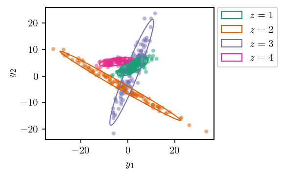

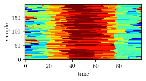
# Plot the number of points associated to each component at each sampling step.
z_hat = categorical2multinomial(chain['z'])
K_hat = z_hat.sum(1)
plt.figure(figsize=(4,2.5))
plt.imshow(K_hat.T,cmap='Greys',extent=[1,z_hat.shape[0],.5,.5+K_hat.shape[-1]])
plt.ylabel(r"component $z$")
plt.xlabel("step")
plt.yticks(np.arange(14)+1)
plt.colorbar(label="count")
plt.tight_layout()
plt.show()

Switching Linear Dynamical System

Switching linear dynamical systems are temporal models that have both a discrete state (HMM) and a continuous state (LDS/Kalman filter). In the example "slds_ex.py" in the examples folder, an SLDS is fit to 1D time-series data. The data is a sinusoidal oscillation that has discrete changes in frequency. Given the data (circles in picture below), Gibbs sampling infers all latent variables and parameters of the model: HMM state "z", LDS state "x", LDS parameters for each discrete state "A,Q,C,R,m0,P0", and HMM parameters "Gamma, pi".

---

Author: Julian Neri
Affil: McGill University
Date: September 2023