Fokker-Planck: Python module for numerical solution, calculation of spectra, and parameter inference for the 1D Fokker-Planck equation
This python module contains tools for working with the one-dimensional Fokker-Planck equation

where P(x,t|x0,t0) is the transition probability density to be at point x at time t, given that one started with delta-peak initial condition P(x,t0|x0,t0) = δ(x-x0) at point x0 at time t0. Furthermore, D(x,t), a(x,t) are the diffusivity and drift profile.
Currently implemented features are
- Parameter inference for time-independent diffusivity D(x) and drift a(x) from given realizations of the Langevin equation corresponding to Eq. (1) [1].
- Numerical calculation of the spectrum of the Fokker-Planck operator defined by the right-hand side of Eq. (1), for various boundary conditions (absorbing, no-flux/reflecting, periodic).
- Numerical simulation of Eq. (1) on a finite domain for various boundary conditions (absorbing, no-flux/reflecting, periodic, general robin boundary conditions) [2].
To install the module fokker_planck, clone the repository and run the installation script:
>> git clone https://github.com/juliankappler/fokker-planck.git
>> cd fokker-planck
>> pip install .In the following we give some short examples of how the module is used. See the folder examples/ for more detailed example notebooks.
Parameter inference is based on calculating the first two Kramers-Moyal coefficients, as explained in detail in Appendix A of Ref. [1]. A detailed inference example is given in this jupyter notebook, here we provide an abbreviated version of that example:
import fokker_planck
# filename of the pickle file that contains the trajectories
trajectories_filename = './sample_trajectories/sample_trajectories.pkl'
# the pickle file should contain a list of 1D arrays, i.e.
# trajectories = pickle.load(open(trajectories_filename,'rb'))
# must lead to an object "trajectories" such that
# trajectories[i] = 1D array
# for i = 0, ..., len(trajectories)
# Note that a sample python script to generate data is provided in
# examples/inference/sample_trajectories
# timestep of the trajectories
dt = 1e-4
# create a dictionary with the parameters
parameters = {'trajectories_filename':trajectories_filename,
'dt':dt}
# create an instance of the kramers_moyal class
inference = fokker_planck.inference(parameters=parameters)
# load the trajectorial data (stored in a pickle file)
inference.load_trajectories()
# before running the inference, we need to create
# an index of the list of trajectories
inference.create_index()
# finally, we run the inference
inference_result = inference.run_inference()
# the call to run_inference returns a dictionary with three 1D arrays:
x = inference_result['x'] # positions
D = inference_result['D'] # diffusivity at the positions x
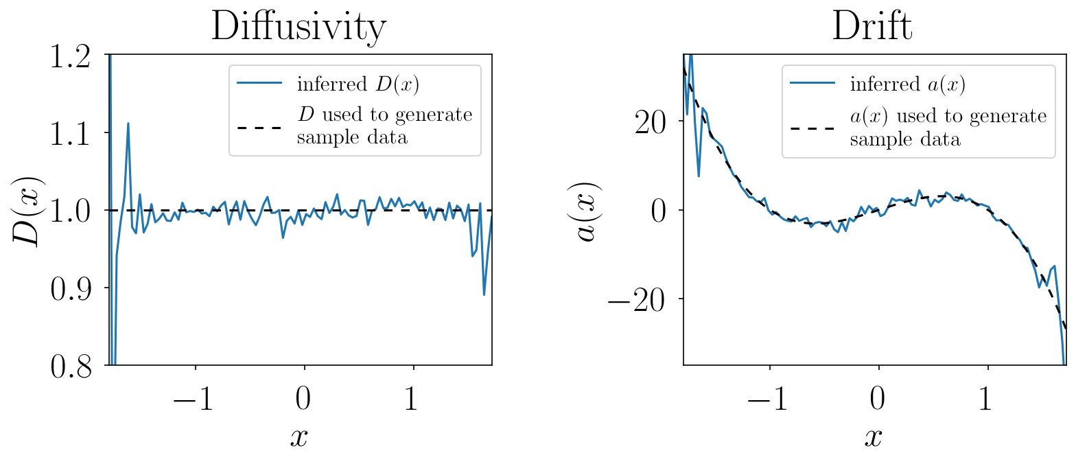
a = inference_result['a'] # drift at the positions xRunning this code on the sample data generated by this script, the inference yields results that compare very well to the diffusivity D(x) = 1 and drift a(x) = -8 · (x2-1) · x used for sample data generation:
The calculation of the slowest-decaying eigenvalues and eigenfunctions of the Fokker-Planck operator uses a spatial discretization. The resulting discretized Fokker-Planck operator is a sparse matrix, the spectrum of which is a discretized approximation to the spectrum of the non-discretized Fokker-Planck operator.
A detailed example which yields approximately the spectrum of the Ornstein-Uhlenbeck process is given in this jupyter notebook; in the following we give an abbreviated version of that example.
import fokker_planck

a = lambda x: -10*x # linear drift, corresponding to quadratic potential
D = 1. # constant diffusivity profile

xl = -2 # left boundary of domain
xr = 2 # right boundary of domain
Nx = 1000 # number of bins for discretization of interval [xl,xr]

# create instance of fokker_planck.numerical class
parameters = {'xl':xl, # left boundary of domain
              'xr':xr, # right boundary of domain
                'Nx':Nx, # number of bins for discretization of interval [xl,xr]
             'boundary_condition_left':'absorbing', # boundary condition at xl
             'boundary_condition_right':'absorbing' # boundary condition at xr
             }
fokker_planck_numerical = fokker_planck.numerical(parameters=parameters)

# Calculate the 4 slowest-decaying eigenfunctions of the system
k = 4
result = fokker_planck_numerical.spectrum(a=a, # drift
                           D=D, # diffusivity
                           k=k) # number of eigenfunctions to calculate

eigenvalues = result['eigenvalues'] # 1D array of length k
eigenvectors = result['eigenvectors'] # 2D array of shape (k, Nx + 2)
x = result['x'] # 1D array of length Nx + 2, contains x-values corresponding to eigenvectors[i]

print(eigenvalues) # prints: array([-1.00804767e-07, -1.00000038e+01, -2.00000680e+01, -3.00007585e+01])
Plotting the resulting eigenvalues and eigenvalues yields:
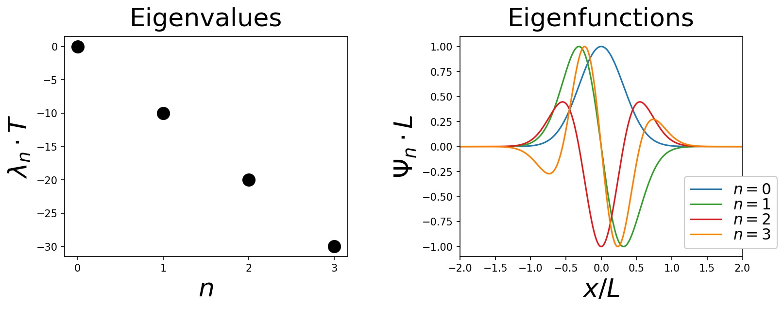
Note that since the drift in this example is very strongly confining the particle to the origin x = 0, the spectrum is on the scales shown in the above plot independent of the boundary conditions. As detailed in in this jupyter notebook, if one calculates the spectrum for reflecting boundary conditions (as opposed to absorbing boundary conditions), one obtains identically looking plots. Of course there are small differences in the two spectra (absorbing/reflecting boundary conditions), which are simply not visible on the scales used for the plots.
[1] Experimental Measurement of Relative Path Probabilities and Stochastic Actions. Jannes Gladrow, Ulrich F. Keyser, Ronojoy Adhikari, Julian Kappler. Physical Review X, vol. 11, p. 031022 (2021). DOI: 10.1103/PhysRevX.11.031022.
[2] Stochastic action for tubes: Connecting path probabilities to measurement. Julian Kappler, Ronojoy Adhikari. Physical Review Research, vol. 2, p. 023407, (2020). DOI: 10.1103/PhysRevResearch.2.023407.