eumaps makes it easy to make professional-quality choropleth maps of the European Union (EU) with only a few lines of code — and without knowing anything about map-making.
eumaps breaks down the process of making a map into three basic steps: (1) specifying the geography to plot, (2) specifying the color palette to use, and (3) specifying a theme that defines the aesthetics of the map.
eumaps includes a wide array of intuitive customization options. It returns a standard ggplot object so you can add labels or other layers.
The data for the country borders comes from Natural Earth, a popular public domain database. This package follows Eurostat in showing Northern Cyprus as part of Cyprus. For all other country borders, this package follows Natural Earth in showing current territorial control.

You can install the latest development version of the eumaps package from GitHub:
# install.packages("devtools")
devtools::install_github("jfjelstul/eumaps@0.1.0")
Important: This package depends on sf, which requires gdal. Follow these instructions to install gdal and the sf package.
If you use the eumaps package to make a map for a project or paper, please cite the package:
Joshua Fjelstul (2021). eumaps: Tools to make maps of the European Union. R package version 0.1.0.
The BibTeX entry for the package is:
@Manual{,
  title = {eumaps: Tools to make maps of the European Union},
  author = {Joshua Fjelstul},
  year = {2021},
  note = {R package version 0.1.0},
}
If you notice an error in the data or a bug in the R package, please report it here.
The main function of the eumaps package is make_map(). The make_map() function has three inputs: an object of the class eumaps.geography created by create_geography() that the specifies geography to plot, an object of class eumap.palette created by create_palette() that specifies the color palette to use, and an object of class eumaps.theme created by create_theme() that specifies the theme. You can also choose a title for your map using title.
The geography input, which needs to be an object of class eumaps.geography created by create_geography(), specifies the geography to plot. The appropriate geography to plot is influenced by which countries are member states on the date of the data, whether the map should center on a subset of member states, the aspect ratio of the map, how zoomed out the map should be, whether the map should include non-member states, whether there should be insets for some member states, and whether the map should use high or low resolution border data. See the section below on creating the geography for more details.
The palette input, which needs to be an object of class eumaps.palette created by create_palette(), specifies a mapping between a continuous variable and a color ramp with a fixed number of colors. It also specifies the colors and labels to use for member states with missing data, for member states where the data is not applicable, and for non-member states. See the section below on creating a color palette for more details.
The theme input, which needs to be an object of class eumaps.theme created by create_theme(), specifies the aesthetics of the map, including the style of the map border, the country borders, the title, the legend, and any insets. See the section below on creating a theme for more details.
The eumaps package makes it easy to customize the look of your map. The functions create_geography(), create_palette(), and create_theme() let you customize nearly every aspect of the map.
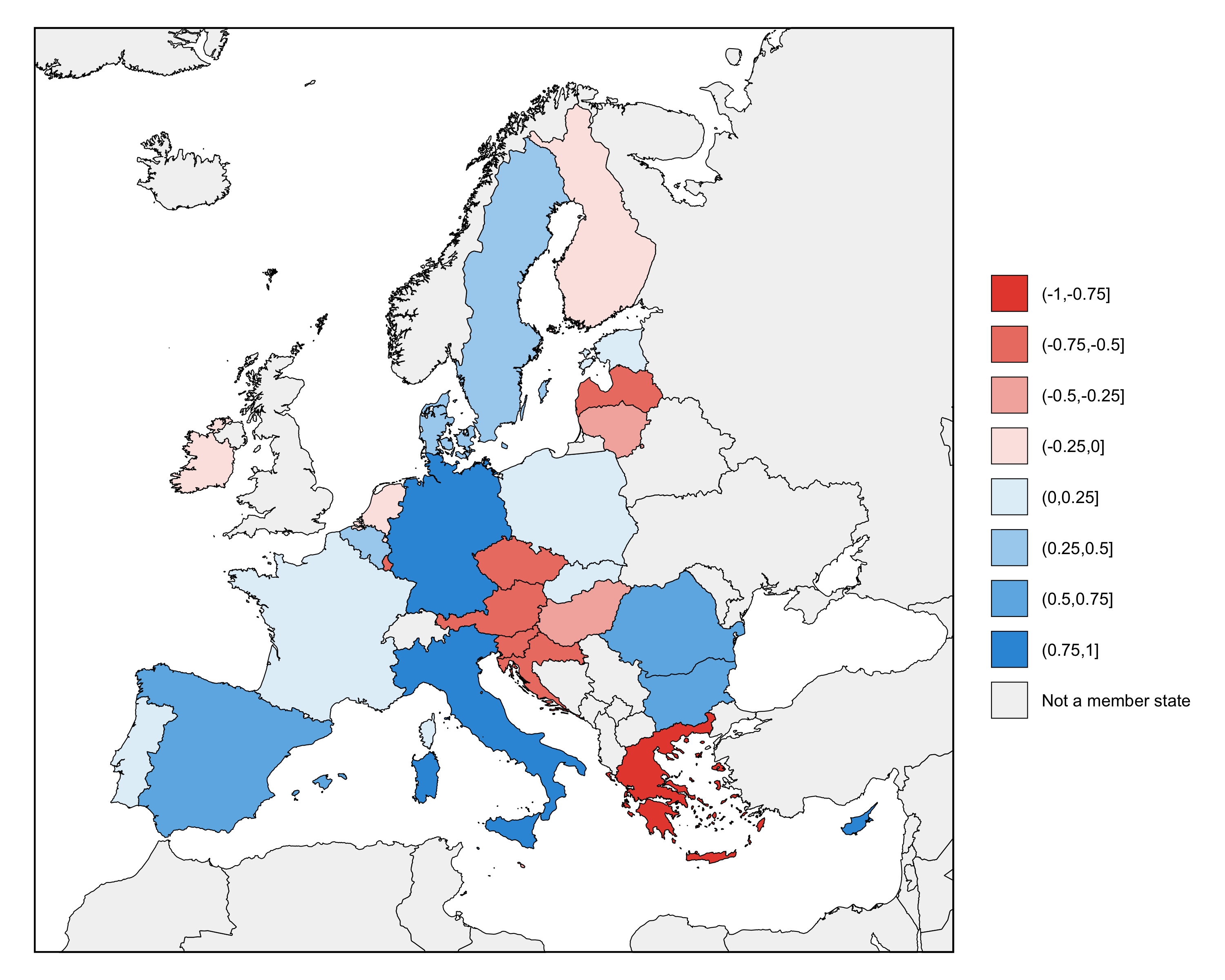
Here's an example of a map with a diverging color palette that uses the default options. This example uses the simulate_data() function to randomly generate fake data. The colors are specified in an RGB format. Note that only create_palette() requires you to choose some values.
# simulate data
data <- simulate_data(
  min = -1,
  max = 1,
  seed = 2468,
)

# make map
map <- make_map(
  geography = create_geography(),
  palette = create_palette(
    member_states = data$member_state,
    values = data$value,
    value_min = -1,
    value_max = 1,
    count_colors = 8,
    color_low = c(231, 76, 59),
    color_high = c(53, 151, 219),
    color_mid = c(255, 255, 255)
  ),
  theme = create_theme()
)
The function create_geometry() creates the geography for a map made by make_map(). It creates a object of type eumaps.geography, which you can pass to the geography argument of make_maps(). You can use create_geography() to set a variety of options that make it easy to make the map look exactly how you want.
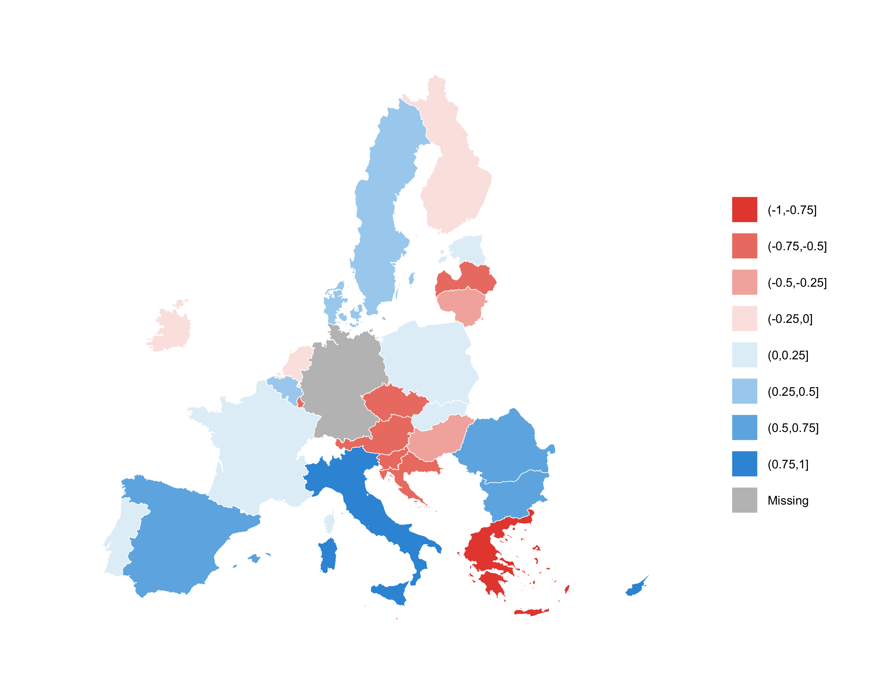
The examples below use the following palette and theme objects. Germany is coded NA to illustrate how missing values are treated.
# simulate data
data <- simulate_data(
  min = -1,
  max = 1,
  missing = "Germany",
  seed = 2468
)

# create palette
palette <- create_palette(
  member_states = data$member_state,
  values = data$value,
  value_min = -1,
  value_max = 1,
  count_colors = 8,
  color_low = c(231, 76, 59),
  color_high = c(53, 151, 219),
  color_mid = c(255, 255, 255)
)

# create theme
theme <- create_theme()
And each map is made using the following code:
# make map
map <- make_map(
  geography = geography,
  palette = palette,
  theme = theme,
)
The only thing that is changing is the geography object.
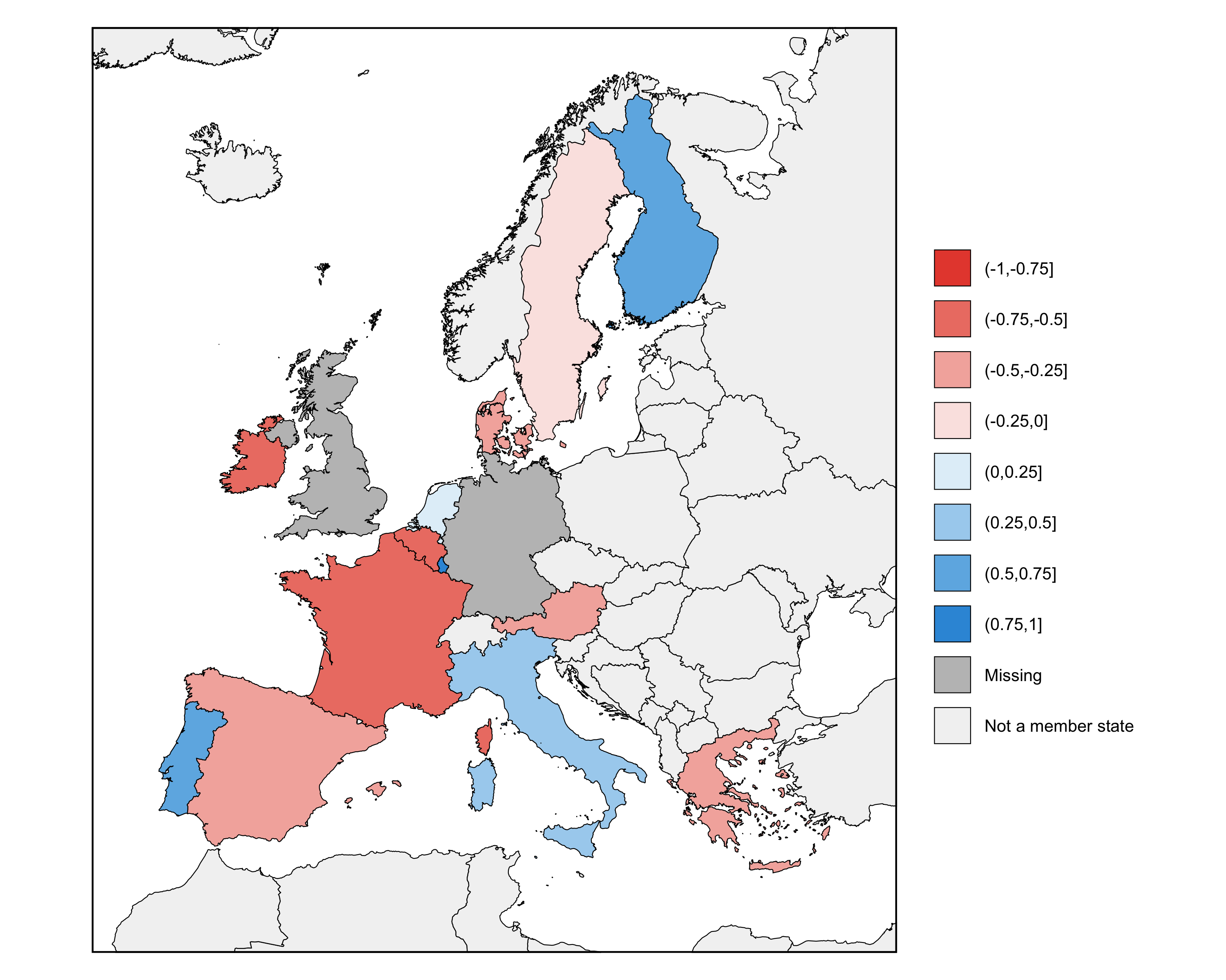
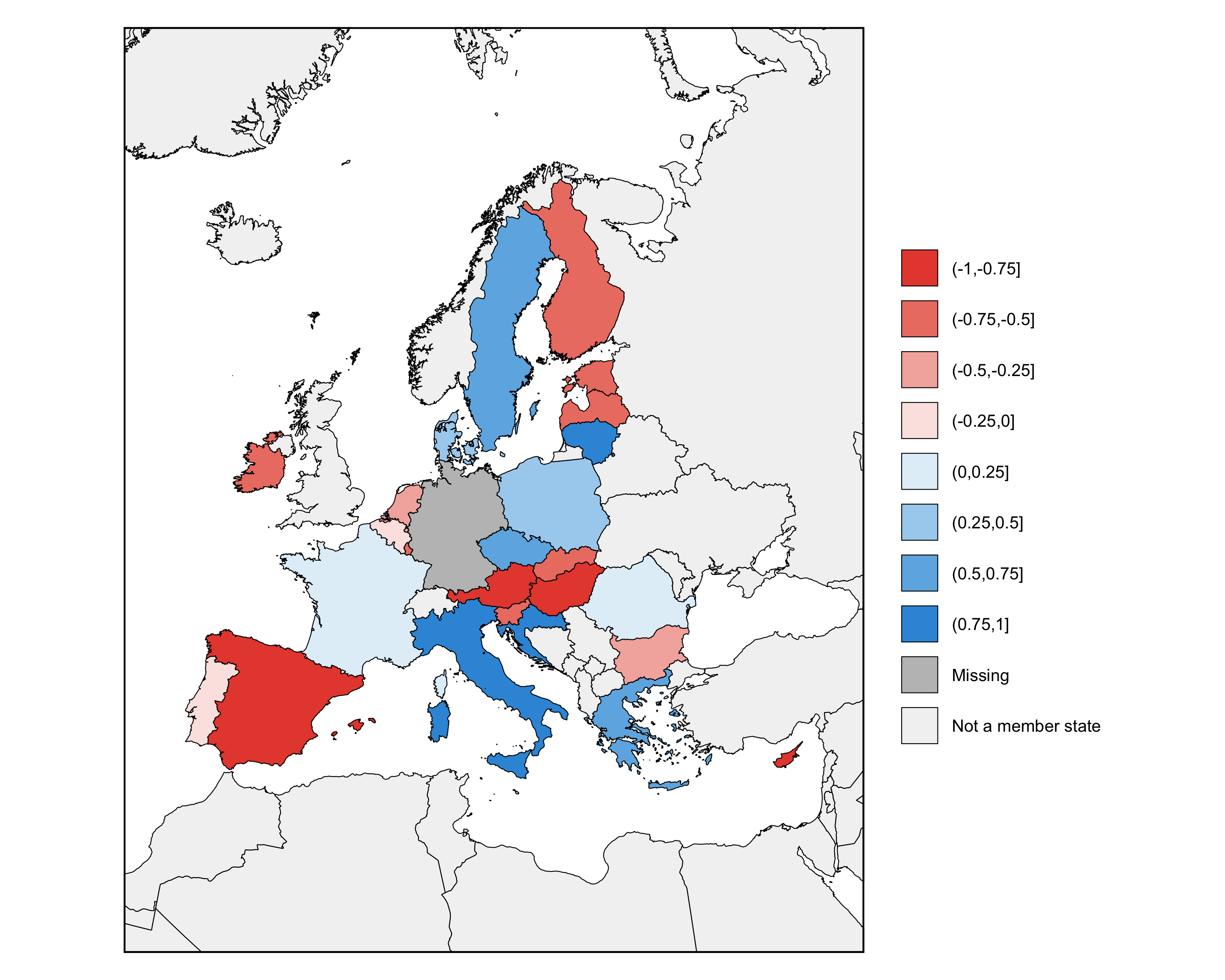
create_geography() will automatically center the map on all countries that are member states on the date indicated by the argument date. This way, you never have to specify the bounds of the map, which can be complicated. You also don't have to know the accession dates of the member states. By default, date is set to today's date. When you use date, data is not plotted for countries that aren't member states on that date. You can use the optional argument subset to center the map on a subset of member states. Data is still plotted for member states that are not in the subset.
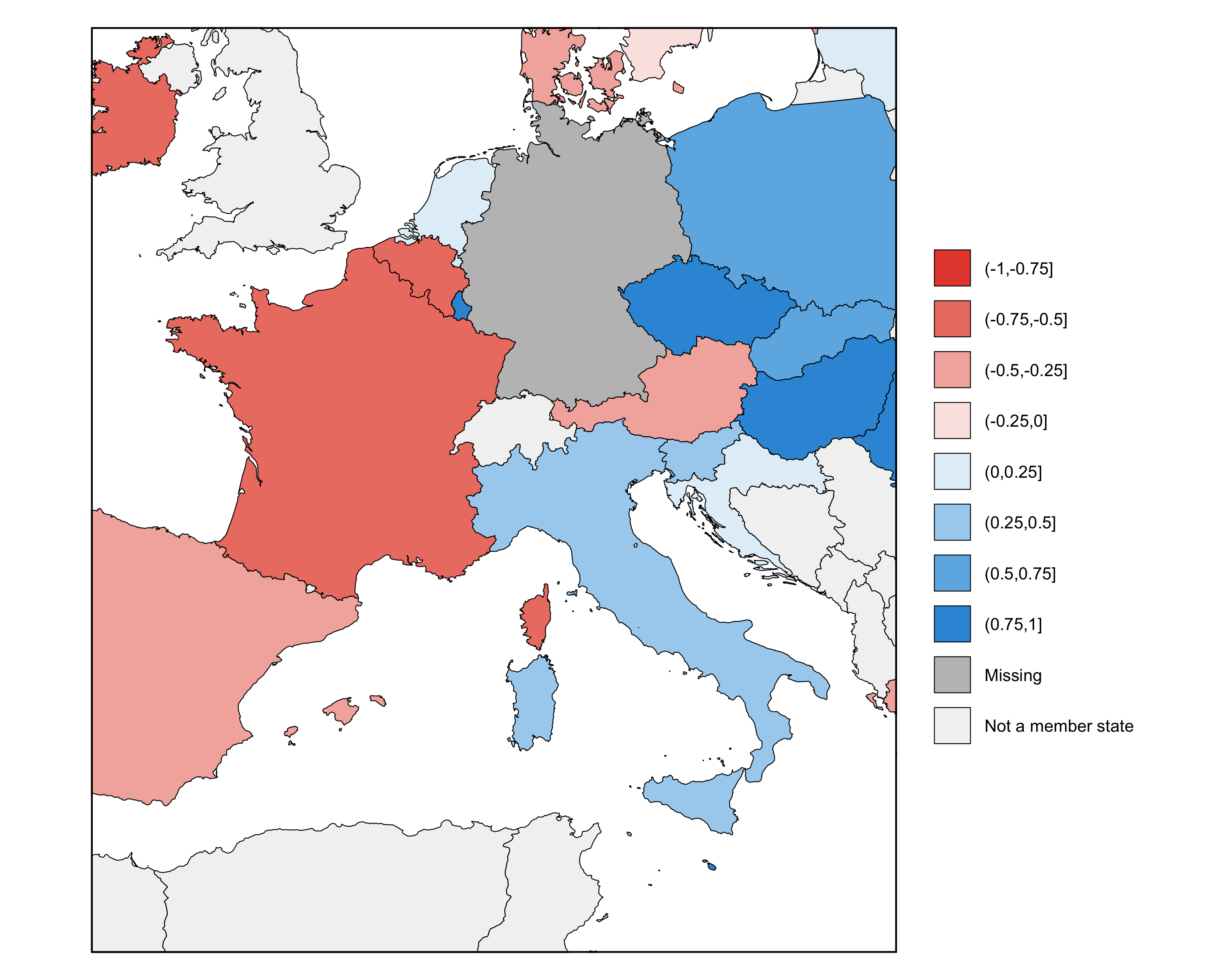
The first example is centered on all current member states, the second is centered on all member states on 2000-01-01, and the third is centered on all member states on 1960-01-01, and the fourth is centered on a subset containing the original member states (France, Germany, Italy, Belgium, the Netherlands, and Luxembourg). The difference between the third and fourth examples is that, in the third example, data is plotted just for countries that are member states on 1960-01-01, whereas in the fourth example, data is plotted for all current member states (because the default value of date is today's date), but the map is centered on a subset of them.
# example 1 (using the default values)
geography <- create_geography()

# example 2 (using the default values for all other arguments)
geography <- create_geography(
  date = "2000-01-01"
)

# example 3 (using the default values for all other arguments)
geography <- create_geography(
  date = "1960-01-01"
)

# example 4 (using the default values for all other arguments)
geography <- create_geography(
  subset = c(
    "France", "Germany", "Italy",
    "Belgium", "Netherlands", "Luxembourg"
  )
)

You can use aspect_ratio to specify the aspect ratio of the map. A value greater than 1 makes a map that is wider than it is tall and a value less than 1 makes a map that is taller than it is wide. The minimum value is 0.5 and the maximum value is 2.
The first example shows an aspect ratio of 0.8, and the second shows an aspect ratio of 1.2.
# example 1 (using the default values for all other arguments)
geography <- create_geography(
  aspect_ratio = 0.8
)

# example 2 (using the default values for all other arguments)
geography <- create_geography(
  aspect_ratio = 1.2
)

You can use zoom to choose a zoom factor. A value of 1 focuses the map tightly around the selected member states, and values less than 1 zoom out the map. The minimum value is 0.5. The default is 0.9.
The first example shows a zoom of 0.8, and the second shows a zoom of 0.7.
# example 1 (using the default values for all other arguments)
geography <- create_geography(
  zoom = 0.8
)

# example 2 (using the default values for all other arguments)
geography <- create_geography(
  zoom = 0.7
)

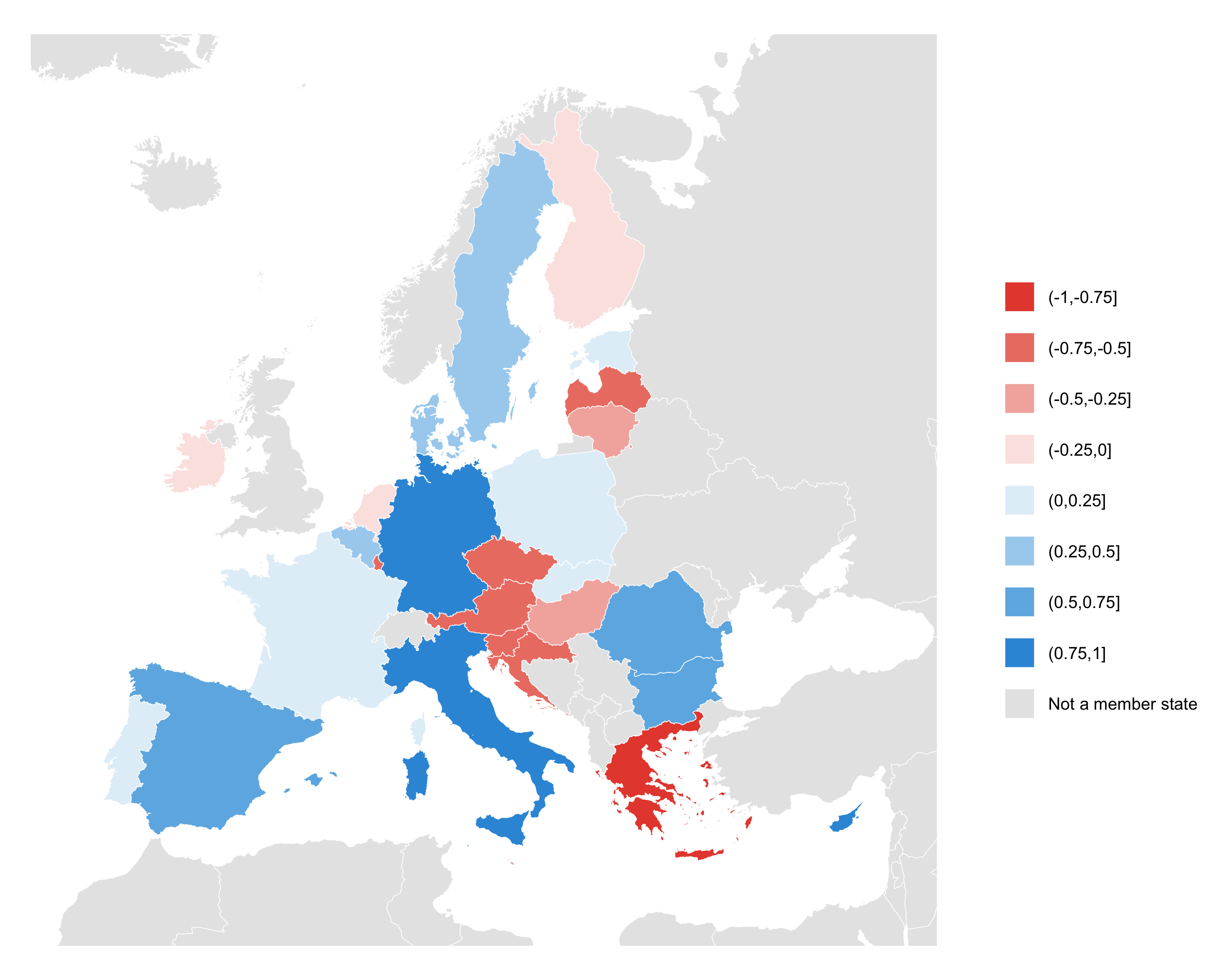
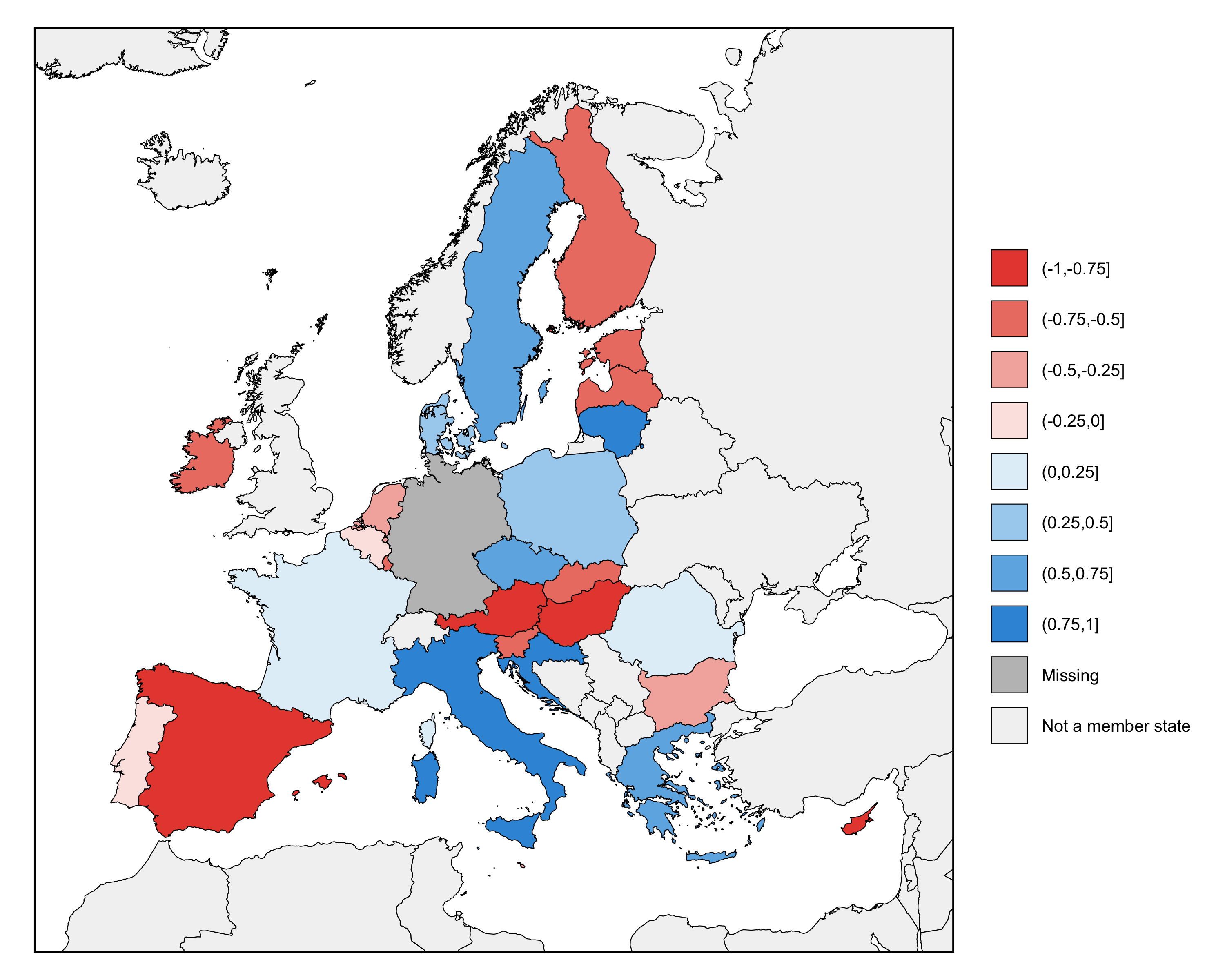
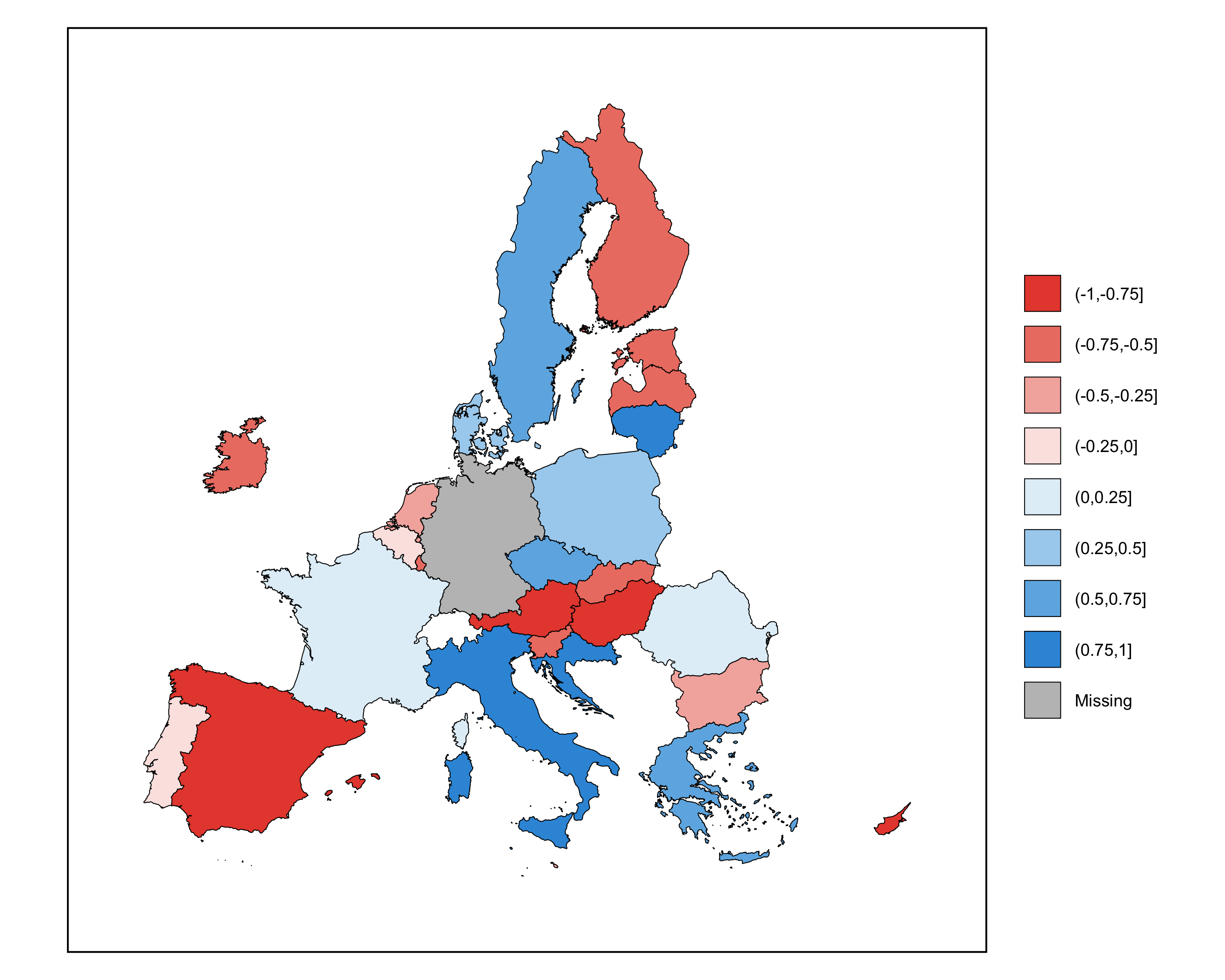
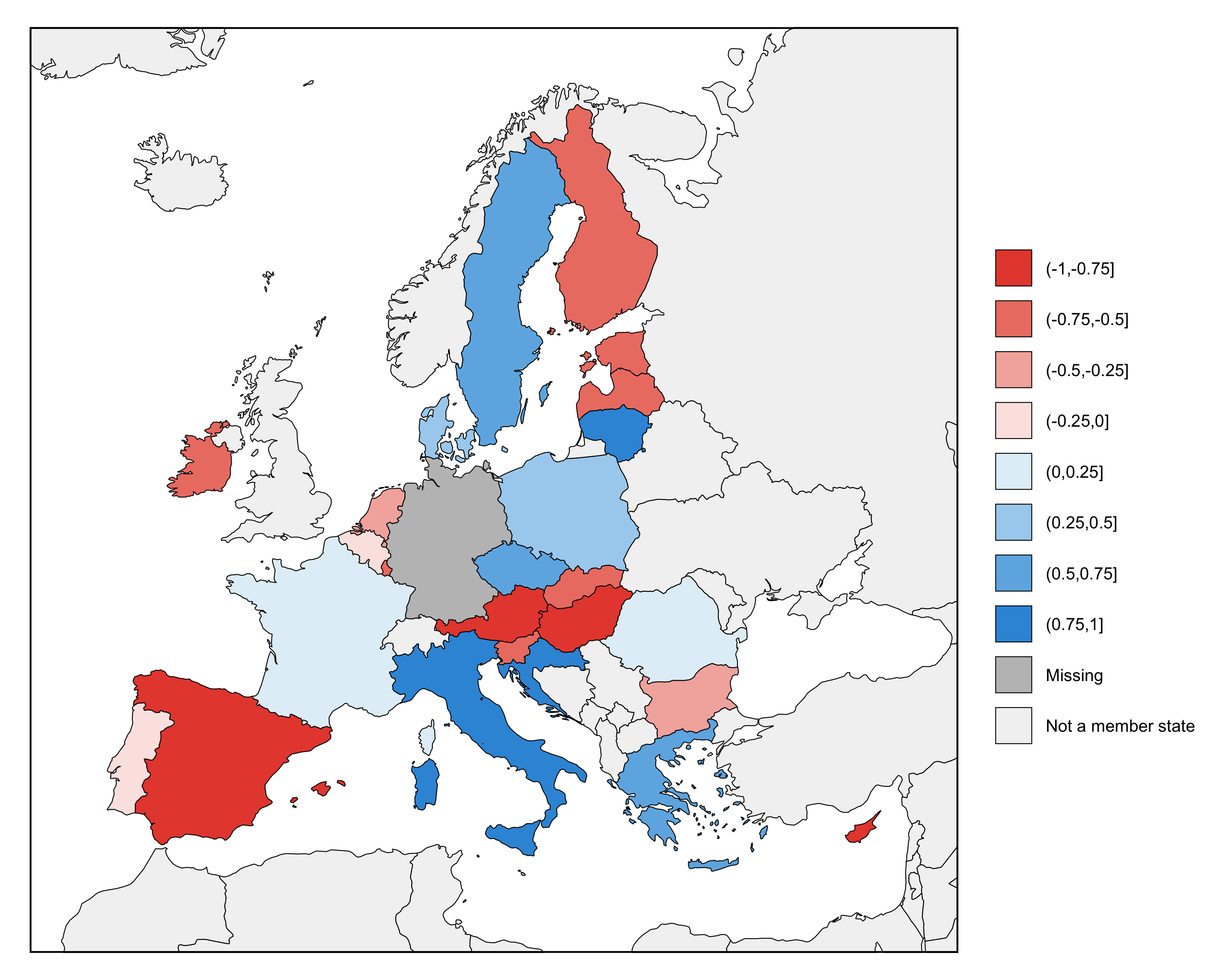
You can use show_non_member_states to choose whether or not to plot non-member states. The default value is TRUE.
The first example shows non-member states, and the second does not.
# example 1 (using the default values for all other arguments)
geography <- create_geography(
  show_non_member_states = TRUE
)

# example 2 (using the default values for all other arguments)
geography <- create_geography(
  show_non_member_states = FALSE
)
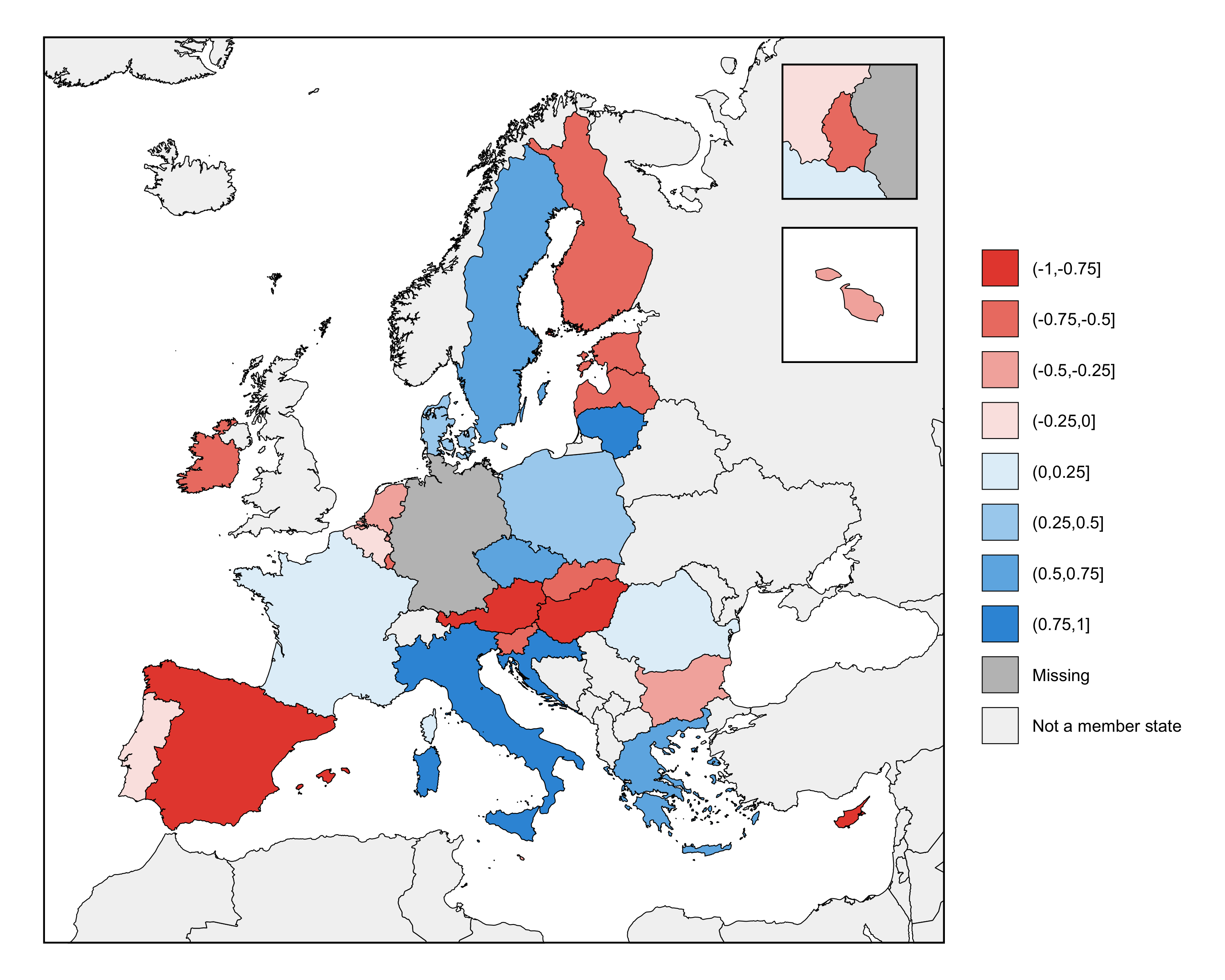
You can use insets to create insets for member states whose values would be hard to read otherwise. By default, insets equals NULL, in which case no insets are created. You can provide a vector of member state names to create insets for those member states. You can create insets for Luxembourg, Malta, and Cyprus. The insets will appear in the top right corner of the map in the order given by the vector.
The first example includes insets for Luxembourg and Malta, and the second includes insets for Luxembourg, Malta, and Cyprus.
# example 1 (using the default values for all other arguments)
geography <- create_geography(
  insets = c("Luxembourg", "Malta")
)

# example 2 (using the default values for all other arguments)
geography <- create_geography(
  insets = c("Luxembourg", "Cyprus", "Malta")
)

You can use resolution to choose between low or high resolution border data. The default value is high and the alternative is low. The map will take longer to render if you use the high resolution data. The function always uses high resolution border data for the insets.
The first example uses the high resolution border data, and the second uses the low resolution data.
# example 1 (using the default values for all other arguments)
geography <- create_geography(
  resolution = "high"
)

# example 2 (using the default values for all other arguments)
geography <- create_geography(
  resolution = "low"
)
The function create_palette() creates the color palette for a map made by make_map(). It creates a object of type eumaps.geography, which you can pass to the palette argument of make_maps(). An eumaps.palette object creates a mapping between a continuous variable and a color ramp with a fixed number of colors. It also defines the colors and labels to use for member states with missing data, member states where the data is not applicable, and non-member states.
Note that an eumaps.palette object only defines the colors used for shading countries on the map. It doesn't define the background color (i.e., the color of the water), the color of country borders, or the color of the border around the map, These are defined using create_theme(), which returns an eumaps.theme object that you can pass to the theme argument of make_map().
create_palette() creates a mapping between a continuous variable and a color ramp with a fixed number of colors. First, you need to provide two vectors: a vector that contains member state names (using the argument member_states) and a vector that contains values corresponding to each member state to be used for shading the member states (using values). Member state names should not be repeated. You can run list_member_states() to get a list of valid member state names.
You can also code certain member states as not applicable (using not_applicable). This is useful in many applications. For example, if you're making a map of the Eurozone, you may only want to plot data for Eurozone members (some of which could have missing data), but still want to visually differentiate between member states that are not members of the Eurozone and countries that are not EU member states. Here, the data would not be applicable for member states that are not members of the Eurozone.
Second, you need to specify minimum and maximum data values (value_min and value_max). These values should be rounded to sensible values, and all of the data points that you want to plot should fall within this range. The function asks you to specify these yourself, instead of calculating the minimum and maximum values in the data (provided via the values argument), because having non-rounded values as the limits of the color ramp doesn't look good. The bounds should either be the theoretical range of the variable you're plotting or rounded values close to the in-sample minimum and maximum values.
Third, you need to specify a low color (color_low) and a high color (color_high) for the color ramp. You also have the option to specify a middle color (color_mid), which lets you to create a diverging color palette. You can speciify colors in an RGB format as a vector, like c(255, 255, 255), or in a hex format as a string, like "#FFFFFF". The leading # is optional. See the documentation for the convert_color() utility function for more details about how you can specify colors.
Fourth, you need to specify the number of colors in the color ramp (count_numbers). There is a limit of 10 colors. Any more than this, and it can become hard to tell them apart, particularly for a linear color ramp. The number of colors in the color ramp determines the number of bins that the data will be divided into. The number of bins is always the same as the number of colors. The break points between the bins will be evenly spaced between the minimum and maximum data values you provide. There is always one fewer break points than the number of colors.
You can also use create_palette() to specify the colors to use for member states with missing data (color_missing), for member states where the data is not applicable (color_not_applicable), and for non-member states (color_non_member_state), along with the labels to use for these three categories in the map legend (label_missing, label_not_applicable, and label_non_member_state). All of these arguments have sensible default values (i.e., shades of gray), so you don't have to specify them every time.
These three colors only appear in the legend when applicable. In other words, color_missing doesn't appear in the legend if there are no missing values, color_not_applicable doesn't appear if not_applicable is set to NULL, and color_non_member_state doesn't appear if non-member states are not plotted (i.e., if show_non_member_states in create_geometry() is set to FALSE).
Here are two examples of how to create a color palette. These maps only show data for Eurozone members, making use of the not_applicable argument. The first example uses a linear color ramp, and the second example uses a divergant color ramp.
data <- simulate_data(
  min = 0,
  max = 1,
  missing = "Germany",
  seed = 1357
)

# example 1 (using the default values for all other arguments)
map <- make_map(
  geography = create_geography(
    insets = c("Luxembourg", "Cyprus", "Malta")
  ),
  palette = create_palette(
    member_states = data$member_state,
    values = data$value,
    not_applicable = c(
      "Bulgaria", "Croatia", "Czech Rebpulic",
      "Denmark", "Hungary", "Poland",
      "Romania", "Sweden"
    ),
    value_min = 0,
    value_max = 1,
    count_colors = 8,
    color_low = c(226, 240, 249),
    color_high = c(53, 151, 219),
    label_not_applicable = "Not a member of the Eurozone"
  ),
  theme = create_theme()
)

# simulate data
data <- simulate_data(
  min = -1,
  max = 1,
  missing = "Germany",
  seed = 1357,
)

# example 2 (using the default values for all other arguments)
map <- make_map(
  geography = create_geography(
    insets = c("Luxembourg", "Cyprus", "Malta")
  ),
  palette = create_palette(
    member_states = data$member_state,
    values = data$value,
    not_applicable = c(
      "Bulgaria", "Croatia", "Czech Rebpulic",
      "Denmark", "Hungary", "Poland",
      "Romania", "Sweden"
    ),
    value_min = -1,
    value_max = 1,
    count_colors = 8,
    color_low = c(231, 76, 59),
    color_high = c(53, 151, 219),
    color_mid = c(255, 255, 255),
    label_not_applicable = "Not a member of the Eurozone"
  ),
  theme = create_theme()
)

The function create_theme() creates the theme for a map made by make_map(). It creates a object of type eumaps.geography, which you can pass to the theme argument of make_maps(). An eumaps.theme object defines the aesthetics of the map, including the style of the map border, the country borders, the title, the legend, and any insets.
See the documentation for details on all available options.
Here are two examples of how to create a theme. The first example uses the default options, and the second example uses custom options.
# simulate data
data <- simulate_data(
  min = -1,
  max = 1,
  seed = 1357
)

# example 1 (using the default values for all other arguments)
map <- make_map(
  geography = create_geography(),
  palette = create_palette(
    member_states = data$member_state,
    values = data$value,
    value_min = -1,
    value_max = 1,
    count_colors = 8,
    color_low = c(231, 76, 59),
    color_high = c(53, 151, 219),
    color_mid = c(255, 255, 255),
  ),
  theme = create_theme()
)

# example 2 (using the default values for all other arguments)
map <- make_map(
  geography = create_geography(),
  palette = create_palette(
    member_states = data$member_state,
    values = data$value,
    value_min = -1,
    value_max = 1,
    count_colors = 8,
    color_low = c(231, 76, 59),
    color_high = c(53, 151, 219),
    color_mid = c(255, 255, 255),
    color_non_member_state = c(0.9, 0.9, 0.9)
  ),
  theme = create_theme(
    color_map_border = c(1, 1, 1),
    width_map_border = 2,
    color_country_borders = c(1, 1, 1),
    width_country_borders = 0.2,
    space_before_legend = 32,
    size_legend_keys = 18,
    space_between_legend_keys = 12
  )
)