This script is intended to be a single-file simple solution to the complex networks degree sequence tail index estimation. It consists of several well-established estimators combined into one toolbox along with some useful plotting routines that usually help to analyze a given degree distribution.
If you use this script as a part of your research, we would be grateful if you cite this code repository and/or the original paper. Real networks data used in the paper can be found in the DegreeSequences directory.
The script requires the following packages to be installed in addition to the standard libraries shipped with Python:
- NumPy
- Matplotlib
No installation is required. Simply download tail-estimation.py file from the directory corresponding to your Python version (either 2 or 3) and use it as demonstrated in the Examples section below.
The script processes a degree sequence in the form of:
k n(k)
where k is a node's degree and n(k) is the number of nodes with such degree in the network. Note that these two numbers are whitespace-separated. User can also provide one of the four supported delimiters using --delimiter flag, see Command Line Options section for more details.
Here we provide the simplest usage example of the tail-estimation script:
python tail-estimation.py <path_to_fomatted_degree_sequence> <path_to_output_file>
Suppose we want to compute the tail exponent of the degree distribution of the CAIDA network provided by KONECT database. Tail exponent is usually denoted by and shows that degree distribution can be described as
. Here
is some slowly-varying function, see the paper for more details.
We first convert the network from the format of an edge list to the format of degree counts as indicated above. The converted data can be found under the Examples directory (CAIDA_KONECT.dat file). Then we run the tail-estimation.py script as follows:
python tail-estimation.py ../Examples/CAIDA_KONECT.dat ./CAIDA_plots.pdf
This will produce a collection of plots saved in the current directory under the "CAIDA_plots.pdf" name as well as some STDOUT messages reporting estimated tail indices. Most users would be interested in just one-number tail index estimates according to three estimators we have implemented so far. They are reported to the STDOUT in the following form (for the CAIDA network example):
Adjusted Hill estimated gamma: 2.09917807967
**********
Moments estimated gamma: 2.11472695937
**********
Kernel-type estimated gamma: 2.10970003848
**********
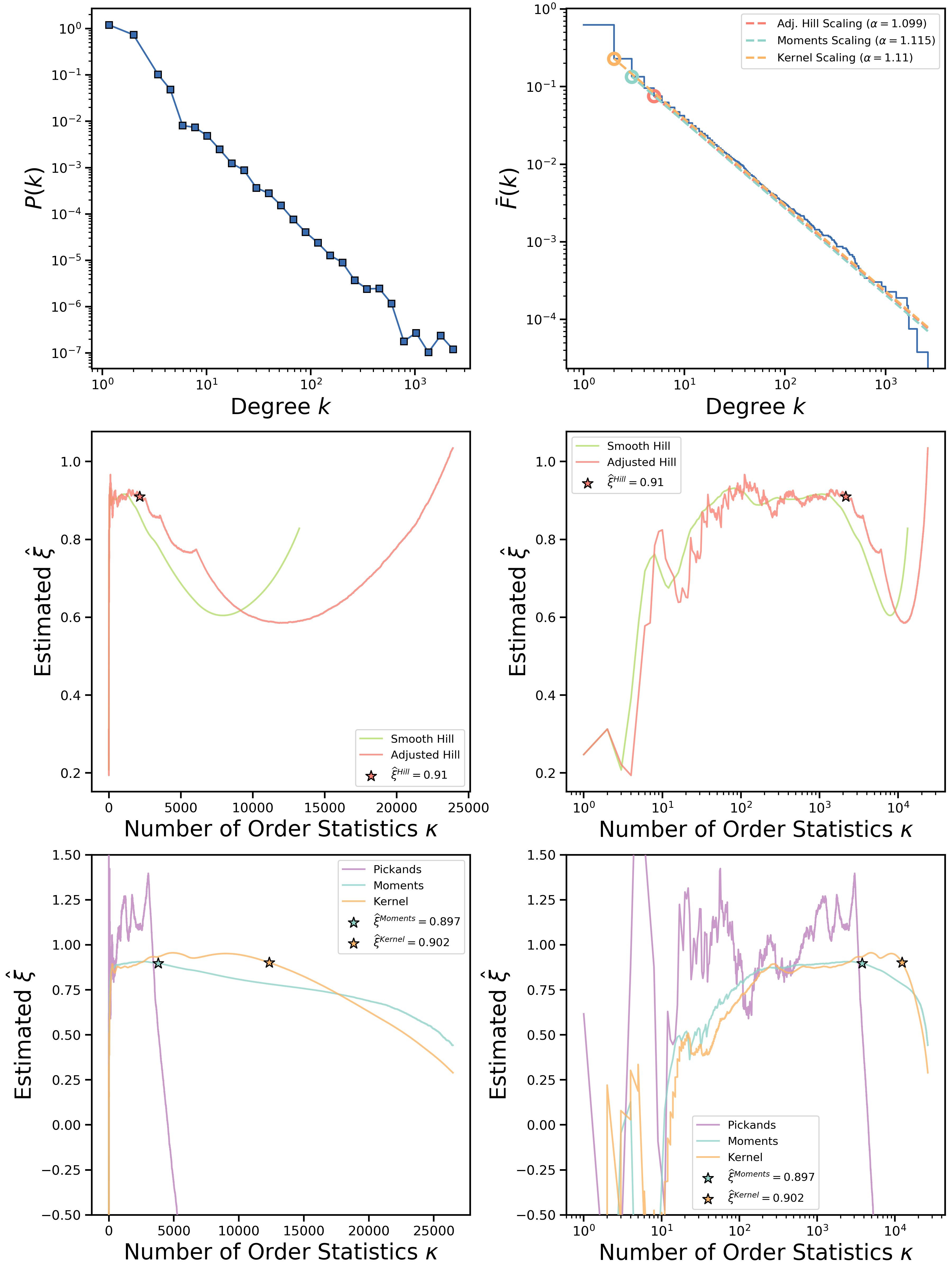
An example of plots generated for the CAIDA network is given below:
Although at the first glance the plots produced by the script may seem to be complicated, it is very easy to interpret them for your network!
The main thing to notice is that all the estimates are plotted in terms of the tail index that is related to the tail exponent of the PDF of degree distribution
as follows:
. We also sometimes use the CCDF tail exponent
.
Here we list the description of what is exactly shown on each subfigure, starting from the top left one:
- Log-binned probability density function (PDF) of a given degree sequence.
- Complementary cumulative distribution function (CCDF) of a given degree sequence along with scalings based on Hill, moments and kernel-type estimates.
- Smooth and adjusted Hill estimates of the
parameter on a linear scale as a function of the number of included degree sequence order statistics
. Star marker shows the best estimate of the tail index
based on the double-bootstrap procedure for Hill estimator.
- Smooth and adjusted Hill estimates of the
- Pickands, moments and kernel-type estimates of the
- Pickands, moments and kernel-type estimates of the
In the simplest example above, three tail index estimators (Hill, moments and kernel-type) give somewhat close values for the degree distribution tail exponent (around 2.1). However, sometimes estimators may disagree with each other. Generally, we recommend to study the CCDF plot of degree distribution closely and look for various artifacts such as sharp tail cutoffs or presence of multiple regions of distribution with different tail exponents. It may also be helpful to study diagnostic plots for double-bootstrap procedure that is used to obtain a single number estimates for the tail index.
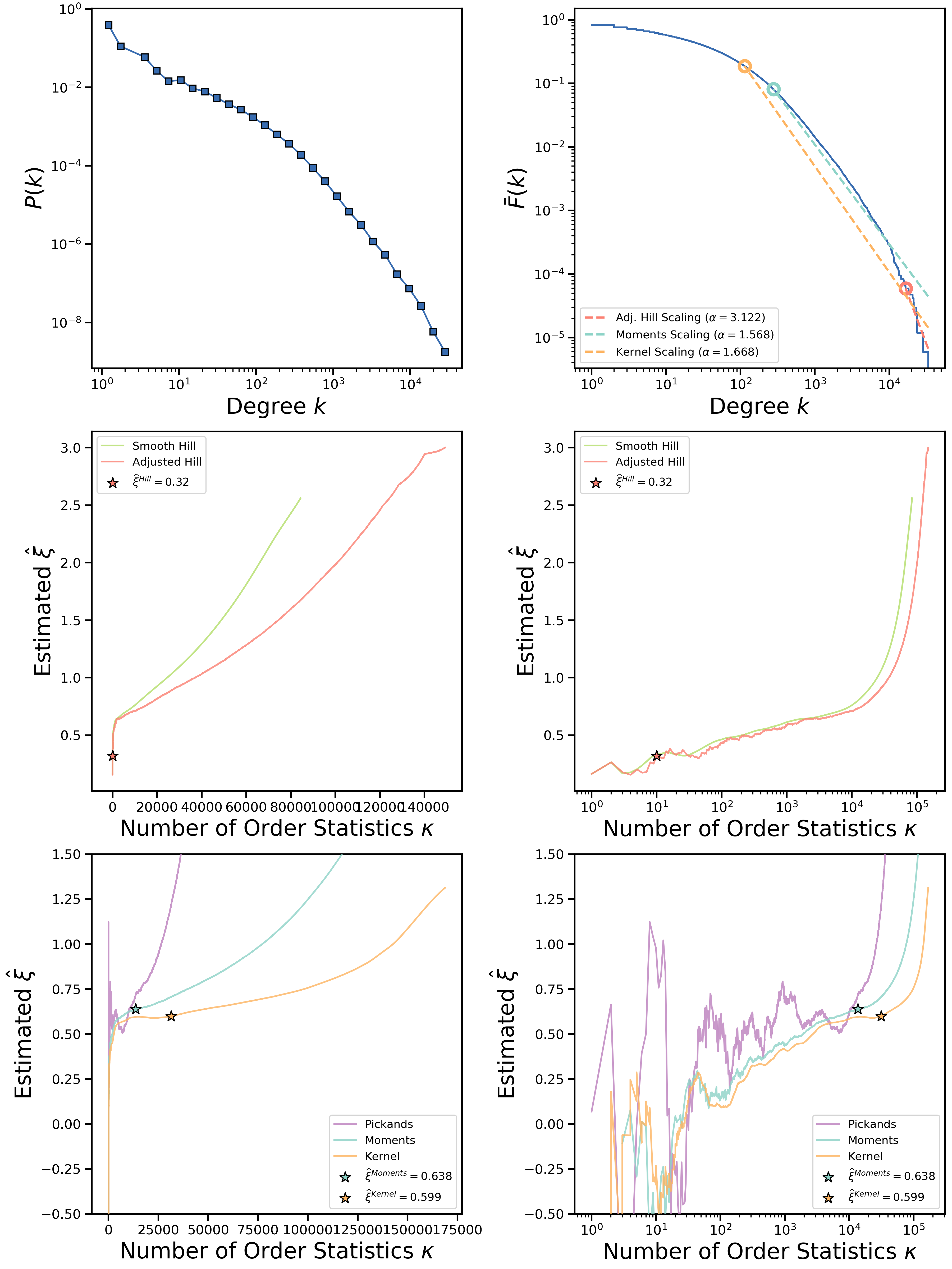
Let us consider an example of in-degree sequence generated from Libimseti dating website network that is also available under the Examples directory (Libimseti_in_KONECT.dat file). Running the script on this sequence produces the following estimates for the tail exponent:
Adjusted Hill estimated gamma: 4.12161848681
**********
Moments estimated gamma: 2.56777932512
**********
Kernel-type estimated gamma: 2.6683297158
**********
While moments and kernel-type estimators produce close estimates, Hill estimator's results is far off from them. From the produced plots we can see that Hill double-bootstrap estimate is placed somewhere very close to the beginning of order statistics of the original sequence, i.e., closer to the tail of the distribution:
This happens due to the features in the landscape of the estimated asymptotic mean-squared error (AMSE) used in the double-bootstrap algorithm. Simply speaking, every double-bootstrap algorithm used for Hill, moments and kernel-type estimators is using two consistent estimators for the tail index for two bootstrap samples of different sizes. The goal of the algorithm is to find the optimal order statistics ,
that correspond to the AMSE minima of the 1st and 2nd bootstrap samples respectively. Based on these two order statistics, the optimal tail index is found. For more details on the double-bootstrap method, please see the paper.
In Hill estimator's case, these two estimators are first- and second-moment tail index estimators; in moments case, these are second- and third-moments estimators; in kernel-type case, these are biweight and triweight kernel-type estimators. The difference between consistent estimators for Hill, moments and kernel-type estimators produce different AMSE landscapes with minima that do not necessarily coincide. This can be seen on the diagnostic plots that can be produced by the script by providing --diagplots 1 in the console as follows:
python tail-estimation.py ../Examples/Libimseti_in_KONECT.dat ./Libimseti.pdf --diagplots 1
This will produce an additional figure that in our case looks like this:
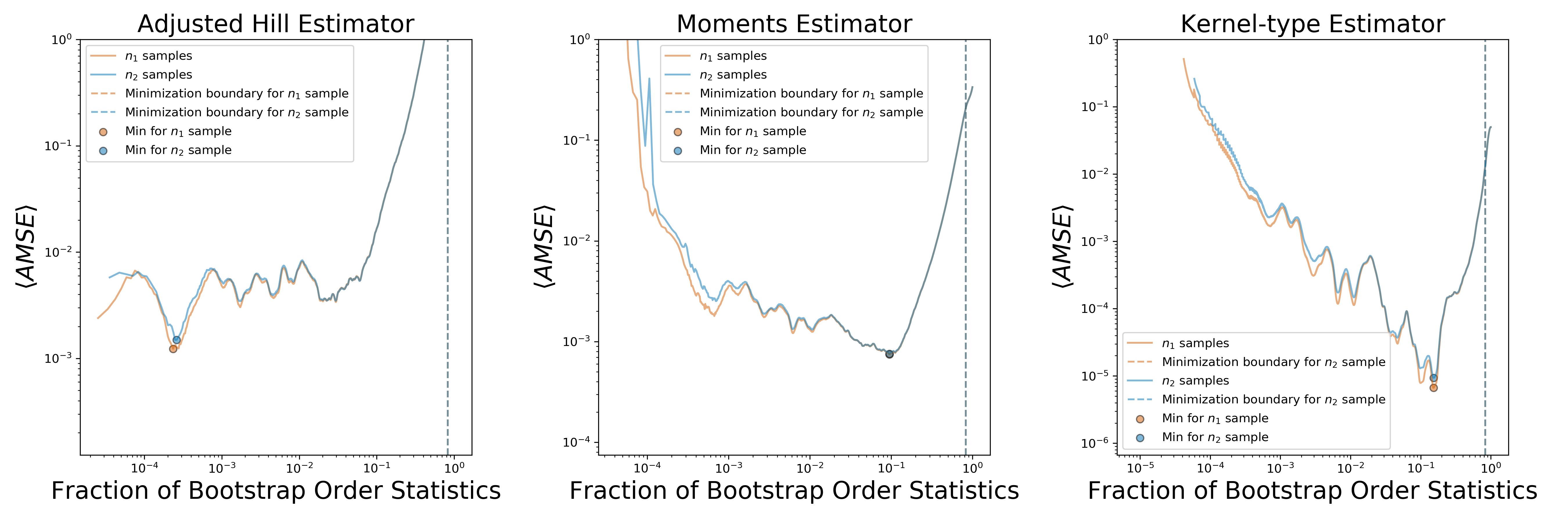
Two subplots show average AMSE plots versus fraction of order statistics used for estimation for three estimators: Hill, moments and kernel-type. Blue and orange lines indicate AMSE lines for the 1st (larger size) and 2nd (smaller size) bootstrap samples; round markers indicate minima for the 1st and 2nd bootstrap samples. Dashed lines indicate boundary after which minimization is not performed. This is done to alleviate problems with artificially added uniform noise that we will describe in details in the next subsection.
As can be seen from the figure, Hill estimator's AMSE plot has minimum somewhere very close to first order statistics which indicates that Hill estimator estimates tail index very close to the actual tail of the empirical distribution. This can be clearly seen on the CCDF plot of the Libimseti in-degree sequence shown on the top right panel of the output figure. Scalings shown by the dashed lines begin from the points where double-bootstrap algorithms "suggest" to start tail index estimation. Clearly, Hill estimator's double-bootstrap suggests to fit only the small fraction of degrees that represent the far tail of the distribution, just as diagnostic plots indicated.
It is known that all estimators used in the package are consistent, however, all consistency proofs are obtained only in certain asymptotic regime, moreover, for real-valued sequences. Working with network degree sequences (that are integer-valued) may possibly worsen estimators' performance. For example, if we consider the same CAIDA network but do not add uniform small noise to each data entry, the resulting plots will look much less converging:
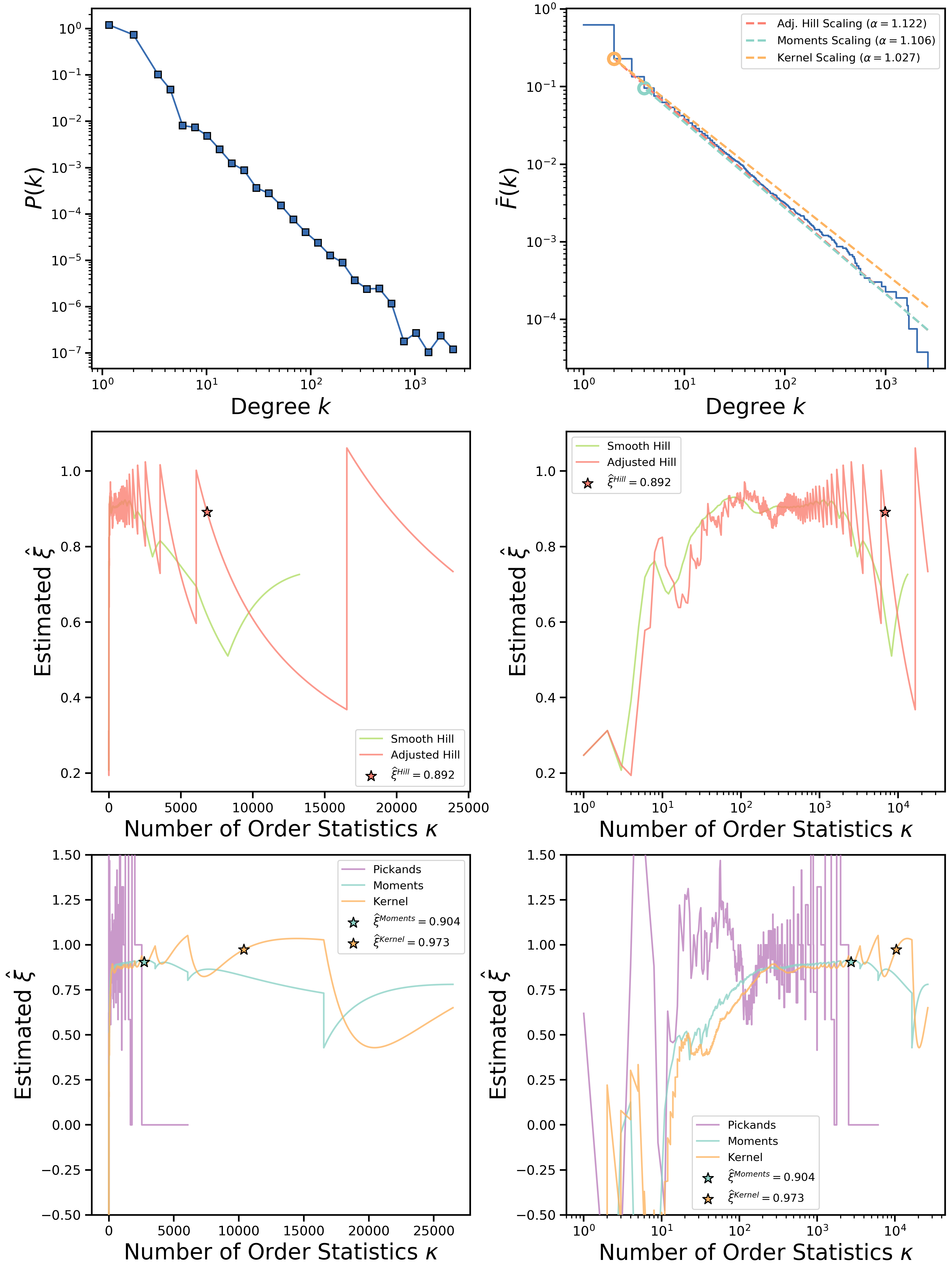
Fortunately, it was shown by J. Velthoen that adding small uniform noise does not affect tail indices of integer-valued distributions, therefore, we apply the same technique in our code. Precisely, we add a small number sampled uniformly from the unit interval to each data entry. Moreover, to prevent double-bootstrap from minimizing in the region of degrees where noise is highly pronounced (i.e., low degrees), we enforce artificial minimization boundary set to the entries less or equal to one. However, it is possible to control this value manually by using --amseborder flag.
It is fairly easy to use our code with non-network data, i.e., non-integer-valued data sequences. Simply convert your data to the required input format and switch off the noise by using --noise 0 flag. We demonstrate this by generating a sequence of Pareto-distributed values with tail exponent . The data sequence converted to the format used by the script can be found under the Examples directory (Pareto.dat file). Estimated tail exponents are very close to the true value:
Adjusted Hill estimated gamma: 2.49891816051
**********
Moments estimated gamma: 2.48997681051
**********
Kernel-type estimated gamma: 2.51013680837
**********
The output plots look as follows for this dataset:
Currently, several estimator are implemented:
- Hill estimator, including smooth Hill estimator;
- moments estimator;
- Pickands estimator;
- kernel-type estimator.
The package implements double-bootstrap estimation of the optimal order statistic for Hill, moments and kernel-type estimators. Details on the double-bootstrap algorithms for these estimators can be found in the following papers:
- Hill double-bootstrap: Danielsson et al. (2001) and Y. Qi (2008);
- moments double-bootstrap: Draisma et al. (1999);
- kernel-type double-bootstrap: Groeneboom et al. (2003).
The script is equiped with a variety of optional arguments that help to study degree sequences in more details. We list all arguments that can be provided to the script in this section.
positional arguments:
  sequence_file_path    Path to a data sequence.

  output_file_path      Output path for plots. Use either PDF or PNG format.

optional arguments:
  -h, --help            show help message and exit

  --nbins               Number of bins for degree distribution (default = 30)

  --rsmooth             Smoothing parameter for smooth Hill estimator (default
                        = 2)

  --alphakernel         Alpha parameter used for kernel-type estimator. Should
                        be greater than 0.5 (default = 0.6).

  --hsteps              Parameter to select number of bandwidth steps for
                        kernel-type estimator, (default = 200).

  --noise               Switch on/off uniform noise in range [-5*10^(-p), 5*10^(-p)]
                        that is added to each data point. Used for integer-valued
                        sequences with p = 1 (default = 1).

  --pnoise              Uniform noise parameter corresponding to the rounding
                        error of the data sequence. For integer values it
                        equals to 1. (default = 1).

  --bootstrap           Flag to switch on/off double-bootstrap algorithm for
                        defining optimal order statistic of Hill, moments and
                        kernel-type estimators. (default = 1)

  --tbootstrap          Fraction of bootstrap samples in the 2nd bootstrap
                        defined as n*tbootstrap, i.e., for n*0.5 a n/2 is the
                        size of a single bootstrap sample (default = 0.5).

  --rbootstrap          Number of bootstrap resamplings used in double-
                        bootstrap. Note that each sample results are stored in
                        an array, so be careful about the memory (default =
                        500).

  --amseborder          Upper bound for order statistic to consider for
                        double-bootstrap AMSE minimizer. Entries that are
                        smaller or equal to the border value are ignored
                        during AMSE minimization (default = 1).

  --theta1              Lower bound of plotting range, defined as k_min =
                        ceil(n^theta1), (default = 0.01). Overwritten if plots
                        behave badly within the range.

  --theta2              Upper bound of plotting range, defined as k_max =
                        floor(n^theta2), (default = 0.99). Overwritten if plots
                        behave badly within the range.

  --diagplots           Flag to switch on/off plotting AMSE statistics for
                        Hill/moments/kernel-type double-bootstrap algorithm.
                        Used for diagnostics when double-bootstrap provides
                        unstable results. Can be used to find proper epsstop
                        parameter. (default = 0).

  --verbose             Verbosity of bootstrap procedure. (default = 0).

  --savedata            Flag to save data files in the directory with plots.
                        (default = 0)

  --delimiter           Delimiter used in the input file. Options are:
                        whitespace, tab, comma, semicolon.