This repository includes the R code that replicates Figure 2-5 of "Trends in men's earnings volatility: What does the Panel Study of Income Dynamics show?" by Shin & Solon (2011, Journal of Public Economics).
The paper studies the change in the earnings volatility of men in the U.S. between 1969 and 2006. To this end, they employ the PSID data for the relevant years. We document the summary statistics of age and wage income distributions, and plot our version of Figure 2 to Figure 5 of the paper.
In Figure 2, we plot these differences. Figure 3 shows the historical movement of the log difference in earnings by plotting 10th, 25th, 50th, 75th and 90th percentile over the entire period. In Figure 4, we compare two methods of calculating volatility of the earnings. Finally, in Figure 5, we plot the 90th percentile-10th percentile difference of the earnings with the latter method in which we use the levels of income rather than the logs.
We provide the list of variables that we use for each year here. The variable names here relates to the variable names as follows:
- 1968 Interview#:
id_68, - Age of HH:
age, - Sex of HH:
gender, - Wage & Sal of HH:
wage, - Accuracy of HH Head Wage:
acc_wage, - Total Labor Income of HH:
inc, - Accuracy of HH Head Labor Income:
acc_inc, - Farm Income of HH:
farm, - Accuracy of Farm Income:
acc_farm, - (Labor Part of) Business Income of HH:
bus, - Accuracy of Business Income:
acc_bus, - Tot. Income Exl Farm and Business HH:
excfarmbus
The list of variables is a collaboration with Lejvi Dalani, Joao Fonsenca Rodrigues, Xiaohan Zhang and Yan Zhao from the Economics Department at University of Minnesota, and myself.
We analyze the two-year differences in earnings throughout the period. So, we prepare a distinct dataset for each pair of years. By doing this, we got 31 datasets: (calendar years) 1969-1971, 1970-1972, 1971-1973, ..., 1994-1996, 1996-1998, ..., 2004-2006. Note that we add 0 to the end of each variable name (except for the 1968 ID) if it's for the initial year, and 1 if it's for the final year. For example, in the data set 1969-1971, we name the initial year's wage as wage0 and the final year's wage as wage1.
We restrict the sample to include only the heads of the households who have the following features:
- gender: male
- age: in [25,59] in both years
- age difference between two years: in {1,2,3}
- belong to: SRC cross-section sample
- wage & total labor income & farm income & business income: not imputed
For Figure 2, 3 and 5, and for the first two plots in Figure 4, we keep the observations only if:
- wage > 1
- total labor income > 1
Then, for all calculations, we drop the top and bottom 1% of the observations:
- wage >= 1st percentile of wages
- wage <= 99th percentile of wages
The summary statistics of ages and wage & salaries in the dataset is as follows:
| Statistic | Age | Wage |
|---|---|---|
| Mean | 38.20 | 29666.51 |
| Median | 37.00 | 24000.00 |
| Std. Dev. | 8.98 | 22958.38 |
| Min | 25.00 | 950.00 |
| Max | 58.00 | 250000.00 |
| Skewness | 0.36 | 2.22 |
| Kurtosis | -0.96 | 8.30 |
| IQR | 15.00 | 24000.00 |
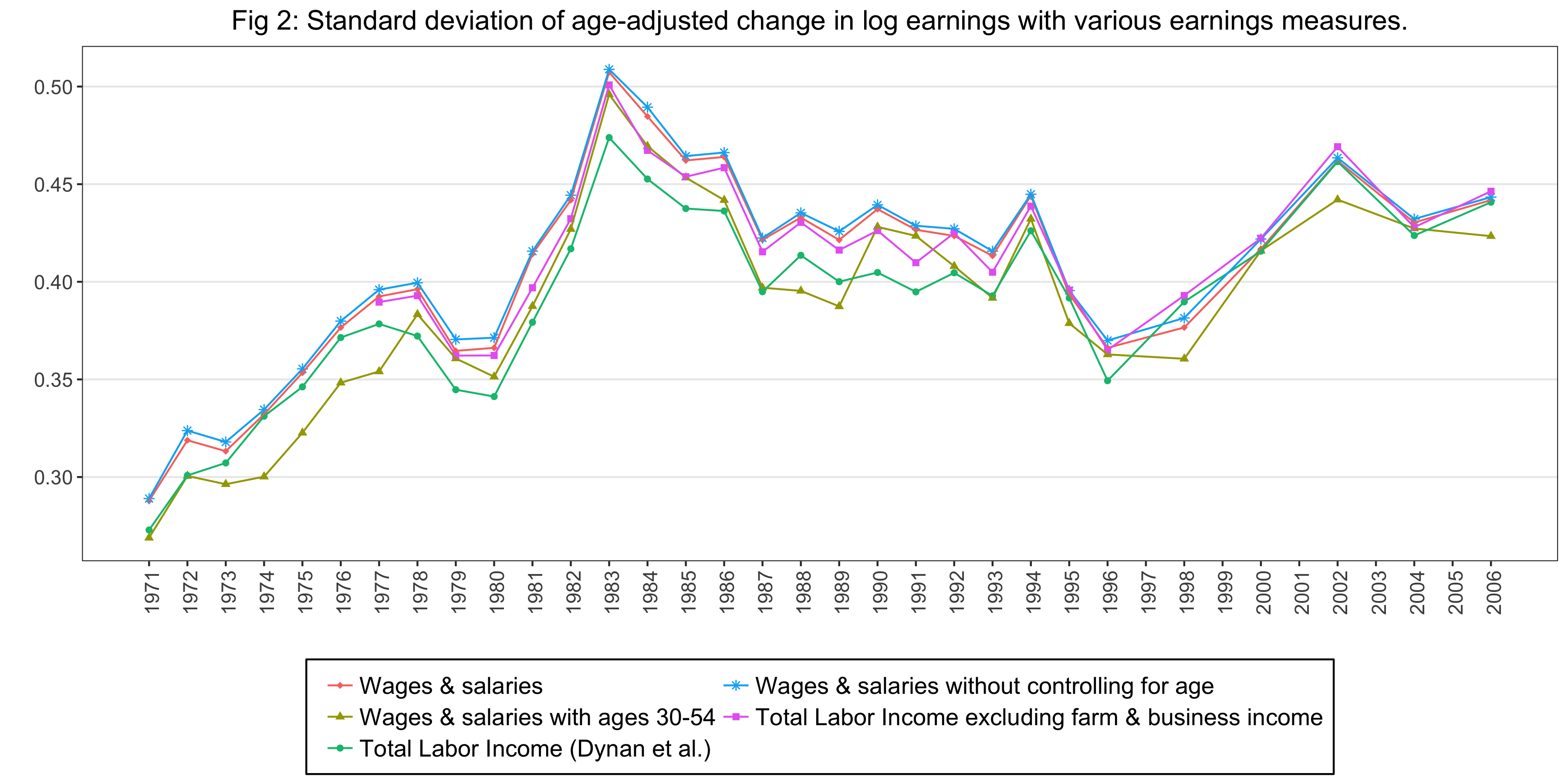
For Figure 2, we calculate the numbers for five series:
- Wages & Salaries: Take the log of the wage and salary income (
wage) for both years, take the difference, regress on a quadratic in age, save the residuals, save the standard deviation of the residuals. - Wages & Salaries with ages 30-54: Restrict the sample to the people at age in [30,54], and do the same as above.
- Total Labor Income (Dynan et al.): Take the log of the total labor income (
inc) for both years, take the difference, regress on a quadratic in age, save the residuals, save the standard deviation of the residuals. - Wages & Salaries without controlling for age: Take the log of the wage and salary income (
wage) for both years, take the difference, save the standard deviation of the difference. - Total Labor Income excluding farm & business income: Take the log of the Total Labor Income excluding farm & business income (
excfarmbus) for both years, take the difference, regress on a quadratic in age, save the residuals, save the standard deviation of the residuals.
Figure 2 is as follows:
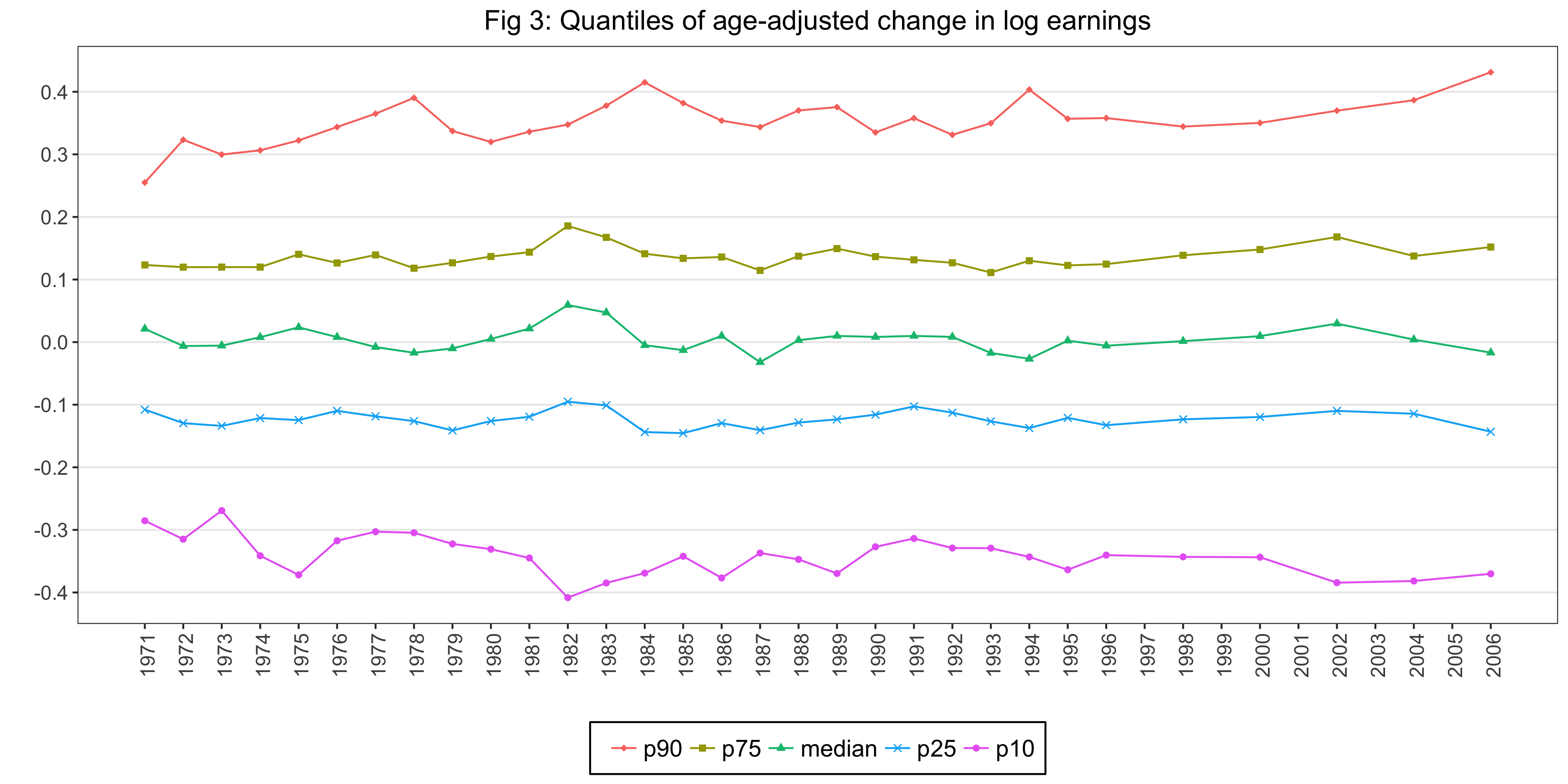
For Figure 3, we take the log of the wage and salary income (wage) for both years, take the difference, regress on a quadratic in age, save the residuals. And then, we calculate the following values:
- p90: 90th percentile of the residuals
- p75: 75th percentile of the residuals
- median: 50th percentile of the residuals
- p25: 25th percentile of the residuals
- p10: 10th percentile of the residuals
Figure 3 is as follows:
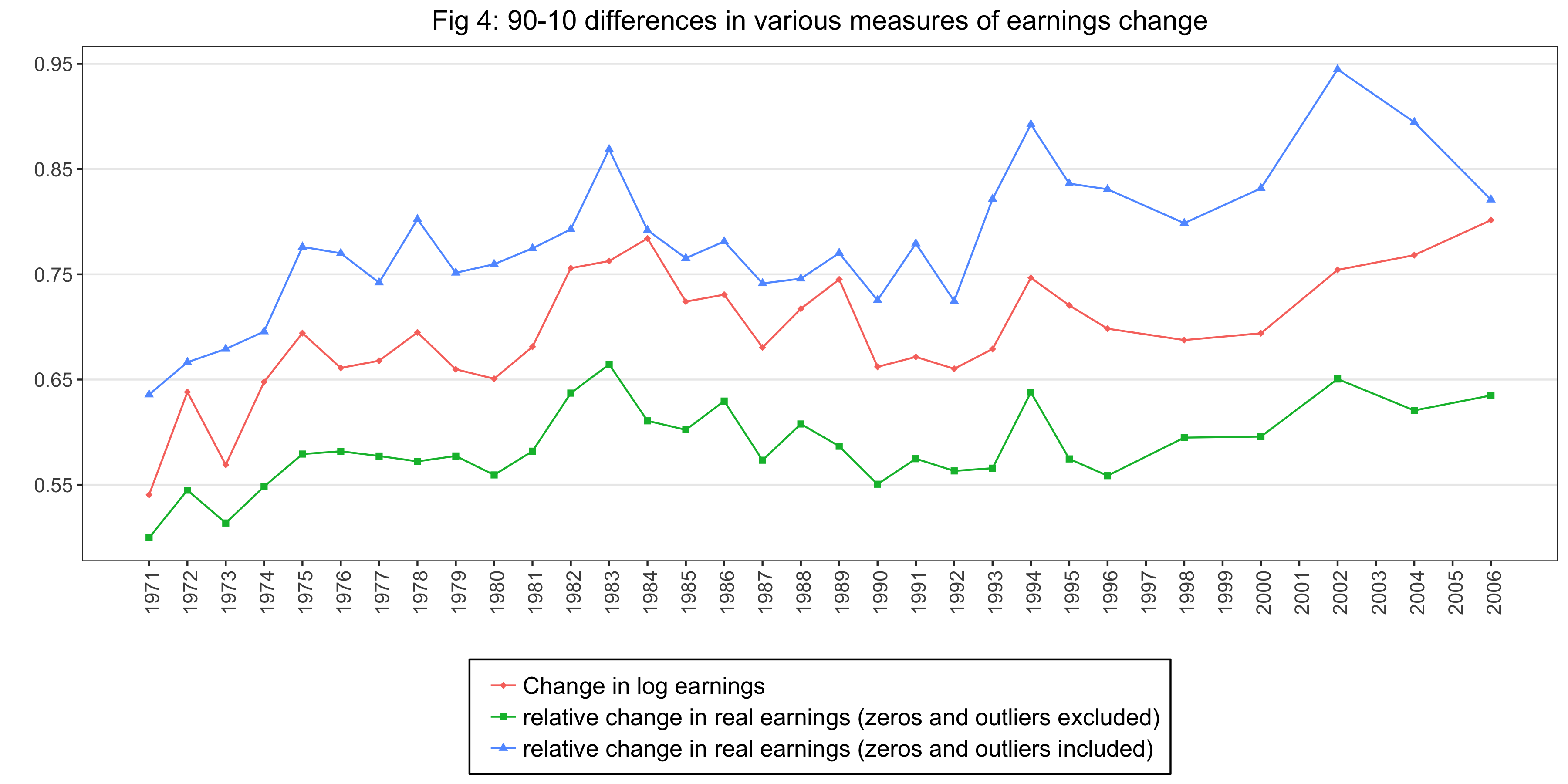
For Figure 4, we calculate the following three series:
- Change in log earnings: Take the log of the wage and salary income (
wage) for both years, take the difference, regress on a quadratic in age, save the residuals, save the standard deviation of the residuals, save the difference between the 90th and the 10th percentile of the residuals. - Relative change in real earnings (zeros and outliers excluded): Here the authors introduce a new method to estimate the earnings change.
"We use the CPI-U-RS to put earnings into real terms. Again we account for the mean effects of year, age, and cohort by estimating a separate regression each year of change in real earnings on a quadratic in age, and then proceed to study the residualized real earnings change. We rescale the residualized real earnings change between years t-2 and t into relative terms by dividing it by the simple average of the sample means of real earnings in the two years." (Shin & Solon, 2011 JPubE)
- Relative change in real earnings (zeros and outliers included): The same calculation described above with the dataset that includes zero earnings.
Figure 4 is as follows:
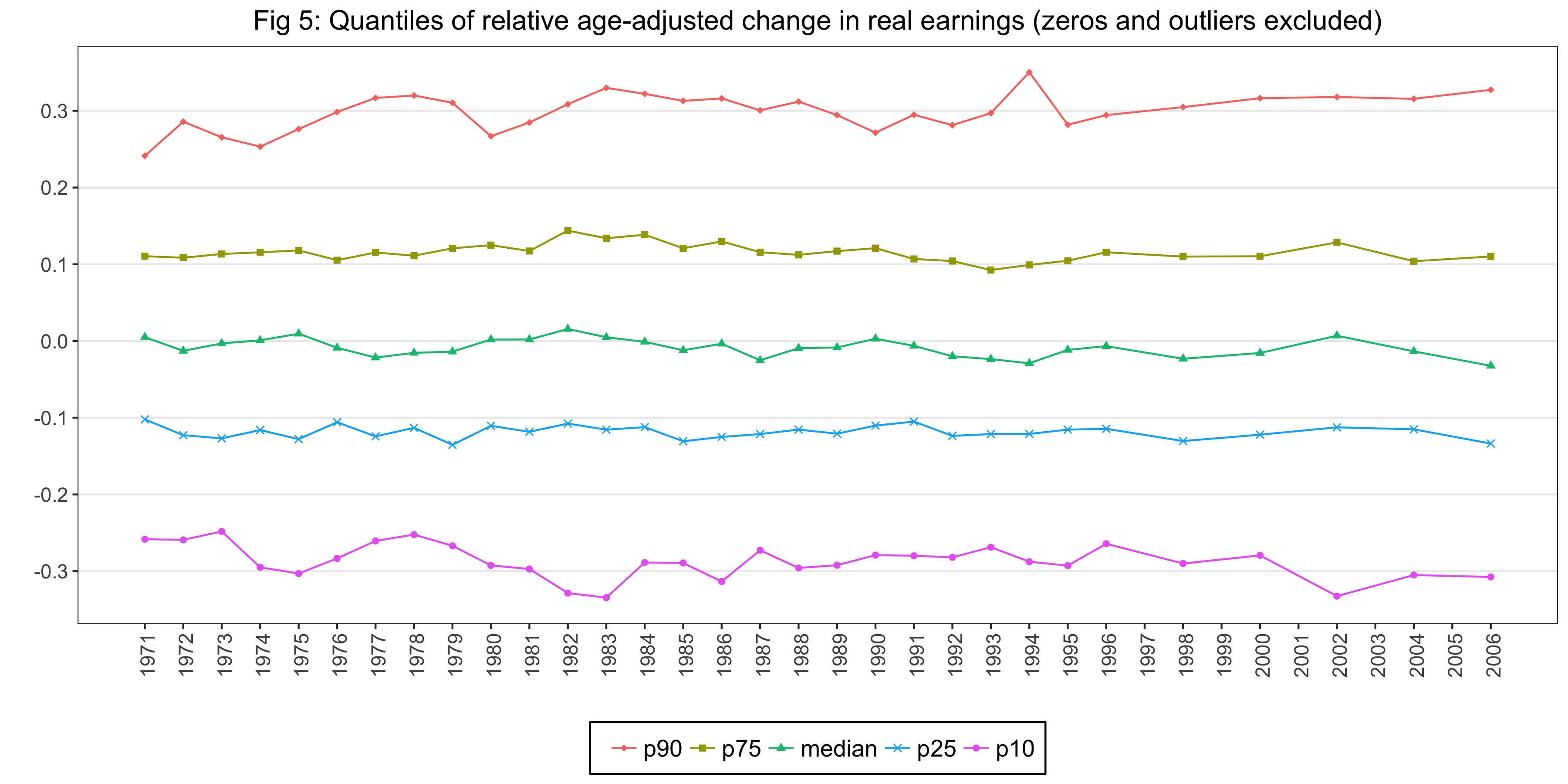
For Figure 5, we do the same calculations as we did for Relative change in real earnings (zeros and outliers excluded) series in Figure 4. Then, we calculate the following five properties of that series:
- p90: 90th percentile
- p75: 75th percentile
- median: 50th percentile
- p25: 25th percentile
- p10: 10th percentile
Figure 5 is as follows: