
Table of Contents
This is a package to convert between one dimensional distance along a Hilbert curve, h, and n-dimensional points, (x_0, x_1, ... x_n-1). There are two important parameters,
n-- the number of dimensions (must be > 0)p-- the number of iterations used in constructing the Hilbert curve (must be > 0)
We consider an n-dimensional hypercube of side length 2^p. This hypercube contains 2^{n p} unit hypercubes (2^p along each dimension). The number of unit hypercubes determine the possible discrete distances along the Hilbert curve (indexed from 0 to 2^{n p} - 1).
Install the package with pip,
pip install hilbertcurveYou can calculate points given distances along a hilbert curve,
>>> from hilbertcurve.hilbertcurve import HilbertCurve
>>> p=1; n=2
>>> hilbert_curve = HilbertCurve(p, n)
>>> distances = list(range(4))
>>> points = hilbert_curve.points_from_distances(distances)
>>> for point, dist in zip(points, distances):
>>>     print(f'point(h={dist}) = {point}')

point(h=0) = [0, 0]
point(h=1) = [0, 1]
point(h=2) = [1, 1]
point(h=3) = [1, 0]
You can also calculate distances along a hilbert curve given points,
>>> points = [[0,0], [0,1], [1,1], [1,0]]
>>> distances = hilbert_curve.distances_from_points(points)
>>> for point, dist in zip(points, distances):
>>>     print(f'distance(x={point}) = {dist}')

distance(x=[0, 0]) = 0
distance(x=[0, 1]) = 1
distance(x=[1, 1]) = 2
distance(x=[1, 0]) = 3The HilbertCurve class has four main public methods.
point_from_distance(distance: int) -> Iterable[int]points_from_distances(distances: Iterable[int], match_type: bool=False) -> Iterable[Iterable[int]]distance_from_point(point: Iterable[int]) -> intdistances_from_points(points: Iterable[Iterable[int]], match_type: bool=False) -> Iterable[int]
Arguments that are type hinted with Iterable[int] have been tested with lists, tuples, and 1-d numpy arrays. Arguments that are type hinted with Iterable[Iterable[int]] have been tested with list of lists, tuples of tuples, and 2-d numpy arrays with shape (num_points, num_dimensions). The match_type key word argument forces the output iterable to match the type of the input iterable.
The HilbertCurve class also contains some useful metadata derived from the inputs p and n. For instance, you can construct a numpy array of random points on the hilbert curve and calculate their distances in the following way,
>>> from hilbertcurve.hilbertcurve import HilbertCurve
>>> p=1; n=2
>>> hilbert_curve = HilbertCurve(p, n)
>>> num_points = 10_000
>>> points = np.random.randint(
        low=0,
        high=hilbert_curve.max_x + 1,
        size=(num_points, hilbert_curve.n)
    )
>>> distances = hilbert_curve.distances_from_points(points)
>>> type(distances)

list

>>> distances = hilbert_curve.distances_from_points(points, match_type=True)
>>> type(distances)

numpy.ndarrayYou can now take advantage of multiple processes to speed up calculations by using the n_procs keyword argument when creating an instance of HilbertCurve.
n_procs (int): number of processes to use
    0 = dont use multiprocessing
   -1 = use all available processes
    any other positive integer = number of processes to use
A value of 0 will completely avoid using the multiprocessing module while a value of 1 will use the multiprocessing module but with a single process. If you want to take advantage of every thread on your computer use the value -1 and if you want something in the middle use a value between 1 and the number of threads on your computer. A concrete example starting with the code block above is,
>>> from hilbertcurve.hilbertcurve import HilbertCurve
>>> p=1; n=2
>>> hilbert_curve = HilbertCurve(p, n, n_procs=-1)
>>> num_points = 100_000
>>> points = np.random.randint(
        low=0,
        high=hilbert_curve.max_x + 1,
        size=(num_points, hilbert_curve.n)
    )
>>> distances = hilbert_curve.distances_from_points(points)
The following methods are able to use multiple cores.
points_from_distances(distances: Iterable[int], match_type: bool=False) -> Iterable[Iterable[int]]distances_from_points(points: Iterable[Iterable[int]], match_type: bool=False) -> Iterable[int]
Due to the magic of arbitrarily large integers in Python, these calculations can be done with ... well ... arbitrarily large integers!
>>> p = 512; n = 10
>>> hilbert_curve = HilbertCurve(p, n)
>>> ii = 123456789101112131415161718192021222324252627282930
>>> point = hilbert_curve.points_from_distances([ii])[0]
>>> print(f'point = {point}')

point = [121075, 67332, 67326, 108879, 26637, 43346, 23848, 1551, 68130, 84004]
The calculations above represent the 512th iteration of the Hilbert curve in 10 dimensions. The maximum value along any coordinate axis is an integer with 155 digits and the maximum distance along the curve is an integer with 1542 digits. For comparison, an estimate of the number of atoms in the observable universe is 10^{82} (i.e. an integer with 83 digits).
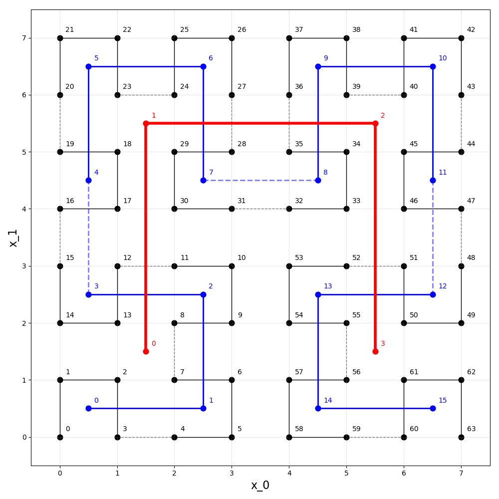
n=2) dimensions. The p=1 iteration is shown in red, p=2 in blue, and p=3 in black. For the p=3 iteration, distances, h, along the curve are labeled from 0 to 63 (i.e. from 0 to 2^{n p}-1). This package provides methods to translate between n-dimensional points and one dimensional distance. For example, between (x_0=4, x_1=6) and h=36. Note that the p=1 and p=2 iterations have been scaled and translated to the coordinate system of the p=3 iteration.
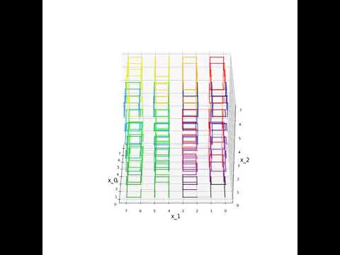
An animation of the same case in 3-D is available on YouTube. To watch the video, click the link below. Once the YouTube video loads, you can right click on it and turn "Loop" on to watch the curve rotate continuously.
This module is based on the C code provided in the 2004 article "Programming the Hilbert Curve" by John Skilling,
- http://adsabs.harvard.edu/abs/2004AIPC..707..381S
I was also helped by the discussion in the following stackoverflow post,
which points out a typo in the source code of the paper. The Skilling code provides two functions TransposetoAxes and AxestoTranspose. In this case, Transpose refers to a specific packing of the integer that represents distance along the Hilbert curve (see below for details) and Axes refer to the n-dimensional coordinates. Below is an excerpt from the documentation of Skilling's code,
//+++++++++++++++++++++++++++ PUBLIC-DOMAIN SOFTWARE ++++++++++++++++++++++++++
// Functions: TransposetoAxes  AxestoTranspose
// Purpose:   Transform in-place between Hilbert transpose and geometrical axes
// Example:   b=5 bits for each of n=3 coordinates.
//            15-bit Hilbert integer = A B C D E F G H I J K L M N O is stored
//            as its Transpose
//                   X[0] = A D G J M                X[2]|
//                   X[1] = B E H K N    <------->       | /X[1]
//                   X[2] = C F I L O               axes |/
//                          high  low                    0------ X[0]
//            Axes are stored conveniently as b-bit integers.
// Author: John Skilling 20 Apr 2001 to 11 Oct 2003Version 2.0 introduces some breaking changes.
Previous versions transformed a single distance to a vector or a single vector to a distance.
coordinates_from_distance(self, h: int) -> List[int]distance_from_coordinates(self, x_in: List[int]) -> int
In version 2.0 coordinates -> point(s) and we add methods to handle multiple distances or multiple points. The match_type kwarg forces the output type to match the input type and all functions can handle tuples, lists, and ndarrays.
point_from_distance(self, distance: int) -> Iterable[int]points_from_distances(self, distances: Iterable[int], match_type: bool=False) -> Iterable[Iterable[int]]distance_from_point(self, point: Iterable[int]) -> intdistances_from_points(self, points: Iterable[Iterable[int]], match_type: bool=False) -> Iterable[int]
The methods that handle multiple distances or multiple points can take advantage of multiple cores. You can control this behavior using the n_procs kwarg when you create an instance of HilbertCurve.