Intro to Machine Learning - kaggle

Summary from article How to build your own Neural Network from scratch in Python

The output ŷ of a simple 2-layer Neural Network is: where W are weights and b are biases, and only these effects the output ŷ. The right values for the weights and biases determines the strength of the predictions. The process of fine-tuning the weights and biases from the input data is known as training.

In each iteration of the training:

• Calculating the predicted output ŷ, known as feedforward
• Updating the weights and biases, known as backpropagation

A way to evaluate the “goodness” of our predictions is the loss function.

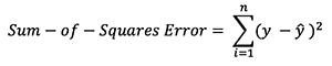
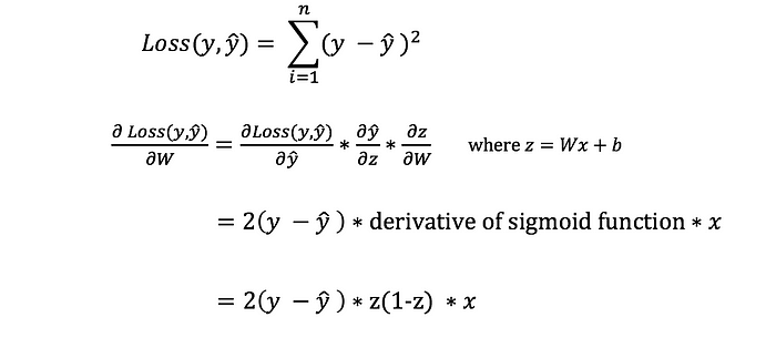
There are many available loss functions, and the nature of our problem should dictate our choice of loss function. In this tutorial, we’ll use a simple sum-of-sqaures error as our loss function: That is, the sum-of-squares error is simply the sum of the difference between each predicted value and the actual value. The difference is squared so that we measure the absolute value of the difference.

Our goal in training is to find the best set of weights and biases that minimizes the loss function.

We need to find a way to propagate the error back, and to update our weights and biases. In order to know the appropriate amount to adjust the weights and biases by, we need to know the derivative of the loss function with respect to the weights and biases. Recall from calculus that the derivative of a function is simply the slope of the function. If we have the derivative, we can simply update the weights and biases by increasing/reducing with it. This is known as gradient descent. However, we can’t directly calculate the derivative of the loss function with respect to the weights and biases because the equation of the loss function does not contain the weights and biases. Therefore, we need the chain rule to help us calculate it.

Our Neural Network should learn the ideal set of weights to represent this function. Note that it isn’t exactly trivial for us to work out the weights just by inspection alone.

code: github.com/jamesloyys/ ... neural_network_backprop-py

basics

from learntools.core import binder
binder.bind(globals())
from learntools.machine_learning.ex2 import *
print("Setup Complete")

import pandas as pd
# Path of the file to read
iowa_file_path = '../input/home-data-for-ml-course/train.csv'

# Fill in the line below to read the file into a variable home_data
home_data = pd.read_csv(iowa_file_path)

# Call line below with no argument to check that you've loaded the data correctly
step_1.check()

• X.describe() - to view summary statistics of the dataset X
• X.head() - to get the fst few rows of dataset, only not empty!
• round(argument) - round the argument to nearest
• home_data["LotArea"].mean() - get the mean of column LotArea

Your First Machine Learning Model

to get columns of dataset:

import pandas as pd

melbourne_file_path = '../input/melbourne-housing-snapshot/melb_data.csv'
melbourne_data = pd.read_csv(melbourne_file_path) 
melbourne_data.columns

# dropna drops missing values (think of na as "not available")
melbourne_data = melbourne_data.dropna(axis=0)

We'll use the . dot notation to select the column we want to predict, which is called the prediction target. By convention, the prediction target is called y. So the code we need to save the house prices in the Melbourne data is

y = melbourne_data.Price

Sometimes, you will use all columns except the target as features. Other times you'll be better off with fewer features. We select multiple features by providing a list of column names inside brackets. Each item in that list should be a string (with quotes). By convention, this data is called X.

melbourne_features = ['Rooms', 'Bathroom', 'Landsize', 'Lattitude', 'Longtitude']

X = melbourne_data[melbourne_features]

Building Your Model

Use sci-kit to create your models.

Building the model in following steps:

1. Define: What type of model will it be?
2. Fit: Capture patterns
3. Predict:
4. Evaluate: determinate the prediction accuracy

example of defining a decision tree:

from sklearn.tree import DecisionTreeRegressor

# Define model. Specify a number for random_state to ensure same results each run
melbourne_model = DecisionTreeRegressor(random_state=1)

# Fit model
melbourne_model.fit(X, y)

Many machine learning models allow some randomness in model training. Specifying a number for random_state ensures you get the same results in each run. This is considered a good practice. You use any number, and model quality won't depend meaningfully on exactly what value you choose.

# Making predictions for the fst 5 houses (X.head())
print(melbourne_model.predict(X.head()))

Model Validation

You've built a model. But how good is it?

You'd first need to summarize the model quality into an understandable way. If you compare predicted and actual home values for 10,000 houses, you'll likely find mix of good and bad predictions. Looking through a list of 10,000 predicted and actual values would be pointless. We need to summarize this into a single metric.

There are many metrics for summarizing model quality, but we'll start with one called Mean Absolute Error (also called MAE). Let's break down this metric starting with the last word, error. This is: error=actual−predicted

# Data Loading Code Hidden Here
import pandas as pd

# Load data
melbourne_file_path = '../input/melbourne-housing-snapshot/melb_data.csv'
melbourne_data = pd.read_csv(melbourne_file_path) 
# Filter rows with missing price values
filtered_melbourne_data = melbourne_data.dropna(axis=0)
# Choose target and features
y = filtered_melbourne_data.Price
melbourne_features = ['Rooms', 'Bathroom', 'Landsize', 'BuildingArea', 
                        'YearBuilt', 'Lattitude', 'Longtitude']
X = filtered_melbourne_data[melbourne_features]

from sklearn.tree import DecisionTreeRegressor
# Define model
melbourne_model = DecisionTreeRegressor()
# Fit model
melbourne_model.fit(X, y)


# calculate the mean absolute error
from sklearn.metrics import mean_absolute_error

predicted_home_prices = melbourne_model.predict(X)
mean_absolute_error(y, predicted_home_prices)

Imagine that, in the large real estate market, door color is unrelated to home price.

However, in the sample of data you used to build the model, all homes with green doors were very expensive. The model's job is to find patterns that predict home prices, so it will see this pattern, and it will always predict high prices for homes with green doors.

Since this pattern was derived from the training data, the model will appear accurate in the training data.

But if this pattern doesn't hold when the model sees new data, the model would be very inaccurate when used in practice.

The most straightforward way to do this is to exclude some data from the model-building process, and then use those to test the model's accuracy on data it hasn't seen before. This data is called validation data.

The scikit-learn library has a function train_test_split to break up the data into two pieces. We'll use some of that data as training data to fit the model, and we'll use the other data as validation data to calculate mean_absolute_error.

from sklearn.model_selection import train_test_split

# split data into training and validation data, for both features and target
# The split is based on a random number generator. Supplying a numeric value to
# the random_state argument guarantees we get the same split every time we
# run this script.
train_X, val_X, train_y, val_y = train_test_split(X, y, random_state = 0)
# Define model
melbourne_model = DecisionTreeRegressor()
# Fit model
melbourne_model.fit(train_X, train_y)

# get predicted prices on validation data
val_predictions = melbourne_model.predict(val_X)
print(mean_absolute_error(val_y, val_predictions))

Underfitting and Overfitting

At the end of this step, you will understand the concepts of underfitting and overfitting, and you will be able to apply these ideas to make your models more accurate.

Set parameters for DecisionTreeRegressor. The most important thng is to set the tree's depth; a tree's depth is a measure of how many splits it makes before coming to a prediction.

If a tree only had 1 split, it divides the data into 2 groups. If each group is split again, we would get 4 groups of houses. Splitting each of those again would create 8 groups. If we keep doubling the number of groups by adding more splits at each level, we'll have 2^10 groups of houses by the time we get to the 10th level. That's 1024 leaves.

This is a phenomenon called overfitting, where a model matches the training data almost perfectly, but does poorly in validation and other new data. On the flip side, if we make our tree very shallow, it doesn't divide up the houses into very distinct groups.

At an extreme, if a tree divides houses into only 2 or 4, each group still has a wide variety of houses. Resulting predictions may be far off for most houses, even in the training data (and it will be bad in validation too for the same reason). When a model fails to capture important distinctions and patterns in the data, so it performs poorly even in training data, that is called underfitting.

The max_leaf_nodes argument provides a very sensible way to control overfitting vs underfitting. The more leaves we allow the model to make, the more we move from the underfitting area in the above graph to the overfitting area.

We can use a utility function to help compare MAE scores from different values for max_leaf_nodes:

from sklearn.metrics import mean_absolute_error
from sklearn.tree import DecisionTreeRegressor

def get_mae(max_leaf_nodes, train_X, val_X, train_y, val_y):
    model = DecisionTreeRegressor(max_leaf_nodes=max_leaf_nodes, random_state=0)
    model.fit(train_X, train_y)
    preds_val = model.predict(val_X)
    mae = mean_absolute_error(val_y, preds_val)
    return(mae)

# Data Loading Code Runs At This Point
import pandas as pd
    
# Load data
melbourne_file_path = '../input/melbourne-housing-snapshot/melb_data.csv'
melbourne_data = pd.read_csv(melbourne_file_path) 
# Filter rows with missing values
filtered_melbourne_data = melbourne_data.dropna(axis=0)
# Choose target and features
y = filtered_melbourne_data.Price
melbourne_features = ['Rooms', 'Bathroom', 'Landsize', 'BuildingArea', 'YearBuilt', 'Lattitude', 'Longtitude']
X = filtered_melbourne_data[melbourne_features]

from sklearn.model_selection import train_test_split
# split data into training and validation data, for both features and target
train_X, val_X, train_y, val_y = train_test_split(X, y,random_state = 0)


# compare MAE with differing values of max_leaf_nodes
for max_leaf_nodes in [5, 50, 500, 5000]:
    my_mae = get_mae(max_leaf_nodes, train_X, val_X, train_y, val_y)
    print("Max leaf nodes: %d  \t\t Mean Absolute Error:  %d" %(max_leaf_nodes, my_mae))

file: exercise-underfitting-and-overfitting.ipynb; Kaggle version kaggle.com/sndorburian

Random Forests

A deep tree with lots of leaves will overfit because each prediction is coming from historical data from only the few houses at its leaf. But a shallow tree with few leaves will perform poorly because it fails to capture as many distinctions in the raw data.

The random forest uses many trees, and it makes a prediction by averaging the predictions of each component tree. It generally has much better predictive accuracy than a single decision tree and it works well with default parameters.

We will use the variables from train_X, val_X, train_y, val_y = train_test_split(X, y,random_state = 0)

We build a random forest model similarly to how we built a decision tree in scikit-learn - this time using the RandomForestRegressor class instead of DecisionTreeRegressor.

from sklearn.ensemble import RandomForestRegressor
from sklearn.metrics import mean_absolute_error

forest_model = RandomForestRegressor(random_state=1)
forest_model.fit(train_X, train_y)
melb_preds = forest_model.predict(val_X)
print(mean_absolute_error(val_y, melb_preds))

There is likely room for further improvement, but this is a big improvement over the best decision tree error of 250,000. There are parameters which allow you to change the performance of the Random Forest much as we changed the maximum depth of the single decision tree. But one of the best features of Random Forest models is that they generally work reasonably even without this tuning.

Conclusion

All in one example: Exercise: Housing Prices Competition: exercise-machine-learning-competitions.ipynb