Fractal Pioneer is a Qt based application for exploring 3D fractals and generating high-FPS high-resolution keyframes from a user defined set of waypoints using a constant speed interpolated camera system. The application was used to generate the above linked YouTube video using a preloaded set of waypoints which are included with the application.
This animation is a screen capture of the application when the Preview Keyframes button is clicked which animates
the preloaded waypoints.
Click on the fractal viewport to capture the keyboard and mouse. Use your mouse to look around. To record your own
custom waypoints uncheck the Use Preloaded Waypoints checkbox on the right and use the hotkeys below.
| Key | Action |
|---|---|
W |
Move forward |
A |
Move sideways (strafe) to the left |
S |
Move backward |
D |
Move sideways (strafe) to the right |
E |
Rotate camera counterclockwise |
Q |
Rotate camera clockwise |
Space |
Record waypoint |
Backspace |
Remove last waypoint |
Delete |
Clear waypoints |
Escape |
Stop animation/preview or stop mouse/keyboard capture |
The tool outputs a sequence of keyframes as PNG images in the desired resolution named in a sequential order. To create a video we can use the the ffmpeg tool to stitch it all together. For example:
ffmpeg -framerate 60 -i %03d.png fractal.mp4
The YouTube video seen above was made using the preloaded waypoints included with the application. The output video was then edited in Premiere Pro to produce the final version seen on YouTube.
The 3D fractal in the Fractal Pioneer application is drawn using a fragment shader (frag.glsl). The fragment which
the fragment shader processes is a simple square covering the canvas where the 3D fractal is drawn. This square is
drawn on an OpenGL Vertex Buffer Object in the resizeGL function. For each pixel on the fragment (our square) the
fragment shader casts a ray from the camera through the pixel to calculate the colour for this pixel.
We use the ray marching method and a distance estimate formula for our fractal to calculate the maximum
distance we can ray march without intersecting the 3D fractal boundary. This process is iterated until we either
reach some defined minimum distance to the fractal or our ray has completely missed the fractal. Depending on the
distance returned by the distance estimator we decide whether to colour the pixel using the background colour or
using the fractal colour at that location. The fractal colour is calculated using orbit traps by the
fractalColour function.
This is all that is needed to draw the 3D fractal. The rest of the code in frag.glsl makes the fractal more visually
pleasing by smoothing it out via anti-aliasing, adding ambient occlusion, fog, filtering, shadows, etc.
The camera position is represented by a 3D vector representing the X, Y, and Z coordinates. The camera rotation is represented by Euler angles which are converted to quaternions for each axis from which we calculate the rotation matrix. Both the position and the rotation matrix are passed to the fragment shader which then uses these values to cast rays from the camera through each pixel and onto the 3D fractal.
When the user clicks on the canvas displaying the fractal we capture the mouse and keyboard and using the defined hotkeys
we apply linear translations to the position via the keyboard and angular translations to the rotation via the mouse. For
example holding the W key will translate the camera forward in the look direction by using the rotation matrix to
extract the look direction vector and apply a scaled vector addition to the current position using the look direction.
For rotations, moving the mouse will result in angular rotation of the Euler angles, which is a simple vector addition.
Camera position and rotation control is implemented in the updatePhysics function.
The application allows the user to record a sequence of waypoints via the addWaypoint function. To animate a
path through the waypoints we have to interpolate the 3D position of the camera. For this we chose to use a
Catmull-Rom spline which has a very simple representation and has the nice property that it interpolates through
the waypoints precisely. The linked whitepaper describes a simple matrix representation to interpolate the spline using
at least four waypoints. The user can of course record as many points as they wish.
The interpolatePosition function implements interpolation of the user defined waypoints as described in the
whitepaper by Christopher Twigg. Catmull-Rom splines require two extra waypoints, called the control points, which
dictate the tangents for the first and the last waypoint. We use the camera look direction to ensure a smooth
animation at the start and end of the spline.
For each recorded waypoint we also record the rotation at that waypoint which we will use to interpolate the rotation of the camera as the position is being interpolated. Unlike the position however, we cannot simply use a spline to interpolate the rotation. Attempting to do so will result in "jerky" camera movement. The reason for this is because 3D rotations form a non-ablian group which can be projected onto a four-dimensional unit sphere of quaternions. Attempting to apply a vector-space interpolation function such as linear interpolation on rotational waypoints will result in camera movement which has non-constant angular momentum. If we project a linear interpolation onto a unit sphere of quaternions, it will be a line between two points on a sphere. The line will cross through the the sphere which is not what we want. This results in the camera rotating slower at the start and end, and fast during the middle of the animation. The mathematics behind this is explained in detail in an excellent whitepaper Quaternions, Interpolation and Animation by Erik B. Dam et. al.
In section 6.2.1. of the whitepaper an interpolation method called Spherical Spline Quaternion interpolation (Squad) of unit quaternions is explored which does a fairly good job at preserving angular momentum while interpolating rotations. As explained in the whitepaper, the Squad algorithm interpolates unit quaternions through a series of waypoints, similar to that of the spline interpolation described in the previous section. Equation 6.14 on pg. 51 defines the interpolation function which is remarkably simple:
Qt does not implement the logarithm and exponential functions for quaternions, so we roll out our own log and
exp functions as defined by Wikipedia. Thankfully the slerp function is implemented by the Qt
QQuaternion class which makes our implementation simple. With that we have all the tools to implement rotational
interpolation using the Squad definitions above. This is implemented in interpolateRotation function by
converting our recorded Euler angle rotational waypoints into unit quaternions and applying the Squad function.
For simplicity let's consider a user recording waypoints in 2D space, and we wish for our camera to interpolate through the user recorded waypoints at a constant velocity. Using a target FPS and a target duration we want the interpolation to last, we can calculate the velocity at which we want the camera to travel.
Consider the following spline with three user recorded waypoints:
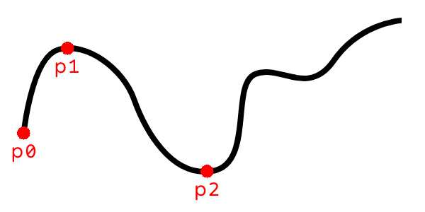
This spline, much like the user recorded waypoints, is defined by a discrete set of points. An obvious first thought to
animate the camera may be to interpolate the camera position between pairs of waypoints,
The problem at hand is that given a sequence of waypoints which define a continuously differentiable spline, how do we interpolate through the spine at a constant velocity?
We know our target FPS and we know the duration we want to take to interpolate the camera through the entirety of the
spline. If we knew the arc length of the spline, we could calculate how far along the spline we need to travel for each
timestep so that our camera velocity would be constant. According to Wikipedia, given a function
If
Thankfully, due to the simplicity of the definition of Catmull-Rom splines as defined in Christopher Twigg's whitepaper,
taking the derivative of takeDerivative parameter in the
interpolatePosition function.
Unfortunately, finding an analytical solution for the integral will not be possible in our case. We must resort to numerical approximations of the integral, which for all intents and purposes will serve us just as well. The canonical numerical integration method I learned through school was using Gaussian quadrature. The Wikipedia article defines the integral equation for us:
using blend.
We are now able to differentiate our position function
Our position interpolation function interpolatePosition takes as input an interpolation parameter
An easy way to solve this problem is to precalculate a table, mapping distances along the spline to interpolation
parameters. We subdivide our spline into small segments by evaluating
The last value in the table will correspond to a reasonably accurate arc length of the entire spline. The table just
described which we call s2uTable is calculated once per animation in the blend function. Moreover we now posses
a way to determine what value of s2u function as a simple binary search.
Finally when the user triggers an animation we use the target FPS to calculate a time delta, we use the target output
duration to calculate the arc length per millisecond that we want to travel, and we use our s2u function to find the
interpolation parameter which will make the camera go the desired distance. All of this is implemented in a few lines
within the updatePhysics function.