
This project set out to examine the Fama-French Three and Five-Factor Models in order to determine which model resulted in the greatest profit. First, a brief background on the Fama-French model (information obtained from https://www.investopedia.com/terms/f/famaandfrenchthreefactormodel.asp):
The first model, the Three-Factor Model, is an asset pricing model developed in 1992 by Nobel laureates Eugene Fame and Kenneth French. It expands on the capital asset pricing model (CAPM) by adding size, risk and value factors to the already established market-risk factor in CAPM. According to the Investopedia article mentioned above, "this model considers the fact that value and small-cap stocks outperform markets on a regular basis. By including these two additional factors, the model adjusts for this outperforming tendency, which is thought to make it a better tool for evaluating manager performance." The three factors are: SMB (Small Minus Big returns), HML (High Minus Low returns) and the portfolio's return minus the risk free rate of return.
In 2014, the duo expanded their model to a 5-Factor Model, adding RMB (Robust Minus Weak returns), a profitability factor, and CMA (Conservative Minus Aggressive returns), an investment factor. In theory, these 2 additional factors should have a beneficial impact on being able to make predictions. Yet, as we will see, there are interesting results when comparing the 3-Factor and 5-Factor returns.
The respective factors for each model were used as features in a Machine Learning model, predictions were generated, and results were evaluated to determine which model, the 3-Factor or the 5-Factor model, was more effective on which to base trading signals. The following ReadMe will depict the results of ATT's stock for the sake of brevity. To see full results of $DIS and $SPY as well, please see "Screenshots" folder.
Please note: This project was created in Google Colab to accomodate for the group, and all code is meant to be run within a Google Colab notebook.
Team members include Ben Fischler, Zachary Green, Priya Roy, Frank Xu and Emmanuel Henao.
In order to more seamlessly progress through the project, we defined various functions that would allow the team to easily read in a CSV and return a cleaned DataFrame:
def get_factors(factors):
  factor_file = factors + ".csv"
  factor_df = pd.read_csv(factor_file)
  factor_df = factor_df.rename(columns={'Unnamed: 0': 'Date'})

  factor_df['Date'] = factor_df['Date'].apply(lambda x: pd.to_datetime(str(x), format='%Y%m%d'))
  factor_df = factor_df.set_index('Date')

  return factor_df
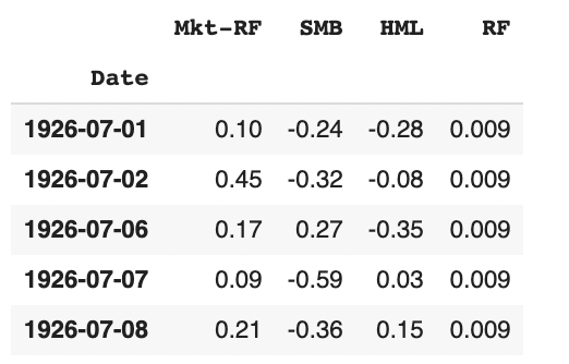
With this "get_factors" function, we were then able to quickly read in any dataframe and not have to manually clean it each time. Using this function resulted in the following Fama-French Three-Factor dataframe from which we were able to work off:
The next function we defined allowed us to the very same thing, but this time, with numbers related to a specific stock's returns as opposed to Fama-French factors:
def choose_stock(ticker):
  ticker_file=ticker+".csv"
  stock=pd.read_csv(ticker_file, index_col='Date', parse_dates=True, infer_datetime_format=True)
  stock["Returns"]=stock["Close"].dropna().pct_change()*100
  stock.index = pd.Series(stock.index).dt.date

  return stock
With this "choose_stock" function, we were then able to quickly read in any dataframe and not have to manually clean it each time. Using this function resulted in the following ATT dataframe from which we were able to work off:

Next, we concatenated the above two dataframes so that we had all of the factors we wanted to use (the 3 Fama-French factors), as well as the target column (Returns) we wanted to use, in the same dataframe:
combined_df = pd.concat([factors, stock], axis='columns', join='inner')
combined_df = combined_df.dropna()
combined_df = combined_df.drop('RF', axis=1)
This gave us the following DataFrame: Mkt-RF, SMB and HML as the 3 factors, and Returns as the target:

We were now prepared to define X/y variables, split into Training/Testing data, and run our Linear Regression using SK Learn:
from sklearn.linear_model import LinearRegression
lin_reg_model = LinearRegression(fit_intercept=True)
lin_reg_model = lin_reg_model.fit(X_train, y_train)
predictions = lin_reg_model.predict(X_test)
We converted y_test to a dataframe using ".to_frame()" and added these predictions to the y_test dataframe. Now came time to generate the signals we would use to backtest our trading strategy, based on the predictions obtained from the 3 Fama-French factors: we decided to "buy" when the day's predicted returns were greater than the day's actual returns, and "sell" when the opposite was true:
y_test['Buy Signal'] = np.where(y_test['Predictions'] > y_test['Returns'], 1.0,0.0)
Now that we had all of this information together in one dataframe, we were able to build on what was already in there, adding new columns showing portfolio performance as time went on. Again, we defined a function to make it easier to change dataframe working off of, starting capital and share count:
def generate_signals(input_df, start_capital=100000, share_count=2000):
  initial_capital = float(start_capital)
  signals_df = input_df.copy()
  share_size = share_count

  # Take a 500 share position where the Buy Signal is 1 (day's predictions greater than day's returns):
  signals_df['Position'] = share_size * signals_df['Buy Signal']

  # Make Entry / Exit Column:
  signals_df['Entry/Exit']=signals_df["Buy Signal"].diff()

  # Find the points in time where a 500 share position is bought or sold:
  signals_df['Entry/Exit Position'] = signals_df['Position'].diff()

  # Multiply share price by entry/exit positions and get the cumulative sum:
  signals_df['Portfolio Holdings'] = signals_df['Close'] * signals_df['Entry/Exit Position'].cumsum()

  # Subtract the initial capital by the portfolio holdings to get the amount of liquid cash in the portfolio:
  signals_df['Portfolio Cash'] = initial_capital - (signals_df['Close'] * signals_df['Entry/Exit Position']).cumsum()

  # Get the total portfolio value by adding the cash amount by the portfolio holdings (or investments):
  signals_df['Portfolio Total'] = signals_df['Portfolio Cash'] + signals_df['Portfolio Holdings']

  # Calculate the portfolio daily returns:
  signals_df['Portfolio Daily Returns'] = signals_df['Portfolio Total'].pct_change()

  # Calculate the cumulative returns:
  signals_df['Portfolio Cumulative Returns'] = (1 + signals_df['Portfolio Daily Returns']).cumprod() - 1

  signals_df = signals_df.dropna()

  return signals_df
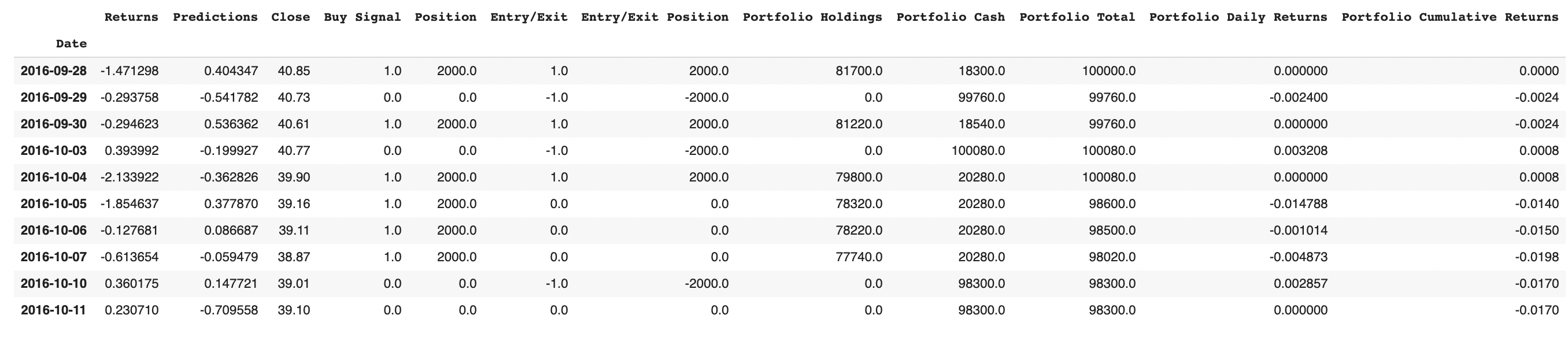
Using this function, we generated our backtested portfolio returns for y_test. This resulted in the following dataframe, which shows important numbers like Portfolio Holdings and Cumulative Portfolio Returns:
Next came time to evaluate the algorithm, and again, we utiliized a custom function to easily calculate different metrics based on which dataframe is read-in:
def algo_evaluation(signals_df):
  # Prepare DataFrame for metrics
  metrics = ['Annual Return', 'Cumulative Returns', 'Annual Volatility', 'Sharpe Ratio', 'Sortino Ratio']

  columns = ['Backtest']

  # Initialize the DataFrame with index set to evaluation metrics and column as `Backtest`:
  portfolio_evaluation_df = pd.DataFrame(index=metrics, columns=columns)

  # Calculate cumulative returns:
  portfolio_evaluation_df.loc['Cumulative Returns'] = signals_df['Portfolio Cumulative Returns'][-1]

  # Calculate annualized returns:
  portfolio_evaluation_df.loc['Annual Return'] = (signals_df['Portfolio Daily Returns'].mean() * 252)

  # Calculate annual volatility:
  portfolio_evaluation_df.loc['Annual Volatility'] = (signals_df['Portfolio Daily Returns'].std() * np.sqrt(252))

  # Calculate Sharpe Ratio:
  portfolio_evaluation_df.loc['Sharpe Ratio'] = (signals_df['Portfolio Daily Returns'].mean() * 252) / (signals_df['Portfolio Daily Returns'].std() * np.sqrt(252))

  #Calculate Sortino Ratio/Downside Return:
  sortino_ratio_df = signals_df[['Portfolio Daily Returns']].copy()
  sortino_ratio_df.loc[:,'Downside Returns'] = 0
  target = 0
  mask = sortino_ratio_df['Portfolio Daily Returns'] < target
  sortino_ratio_df.loc[mask, 'Downside Returns'] = sortino_ratio_df['Portfolio Daily Returns']**2
  down_stdev = np.sqrt(sortino_ratio_df['Downside Returns'].mean()) * np.sqrt(252)
  expected_return = sortino_ratio_df['Portfolio Daily Returns'].mean() * 252
  sortino_ratio = expected_return/down_stdev
  portfolio_evaluation_df.loc['Sortino Ratio'] = sortino_ratio

  return portfolio_evaluation_df
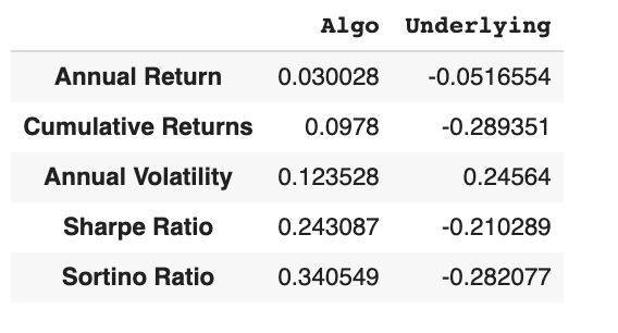
Using this function, we were able to generate an evaluation table for any dataframe we read-in. This is the one for ATT, based on the signals dataframe generated above:

Then we generated the same metrics, but this time, without using our backtested strategy of buy-and-sell; this time, we generated the metrics based on a buy-and-hold strategy to compare how our model did vs. how it would have done should it have simply held throughout:
Last step was to define a function which accepted the daily signals dataframe and returned evaluations of individual trades:
def trade_evaluation(signals_df):
  trade_evaluation_df = pd.DataFrame(
    columns=['Entry Date', 'Exit Date', 'Shares', 'Entry Share Price', 'Exit Share Price', 'Entry Portfolio Holding', 'Exit Portfolio Holding', 'Profit/Loss'])

  entry_date = ''
  exit_date = ''
  entry_portfolio_holding = 0
  exit_portfolio_holding = 0
  share_size = 0
  entry_share_price = 0
  exit_share_price = 0

  # Loop through signal DataFrame. If `Entry/Exit` is 1, set entry trade metrics.  Else if `Entry/Exit` is -1, set exit trade metrics and calculate profit, then append the record to the trade evaluation DataFramefor index, row in signals_df.iterrows():
      if row['Entry/Exit'] == 1:
          entry_date = index
          entry_portfolio_holding = row['Portfolio Total']
          share_size = row['Entry/Exit Position']
          entry_share_price = row['Close']

      elif row['Entry/Exit'] == -1:
          exit_date = index
          exit_portfolio_holding = abs(row['Portfolio Total'])
          exit_share_price = row['Close']
          profit_loss = exit_portfolio_holding - entry_portfolio_holding
          trade_evaluation_df = trade_evaluation_df.append(
              {
                  'Entry Date': entry_date, 'Exit Date': exit_date, 'Shares': share_size, 'Entry Share Price': entry_share_price, 'Exit Share Price': exit_share_price, 'Entry Portfolio Holding': entry_portfolio_holding, 'Exit Portfolio Holding': exit_portfolio_holding, 'Profit/Loss': profit_loss}, ignore_index=True)

  return trade_evaluation_df
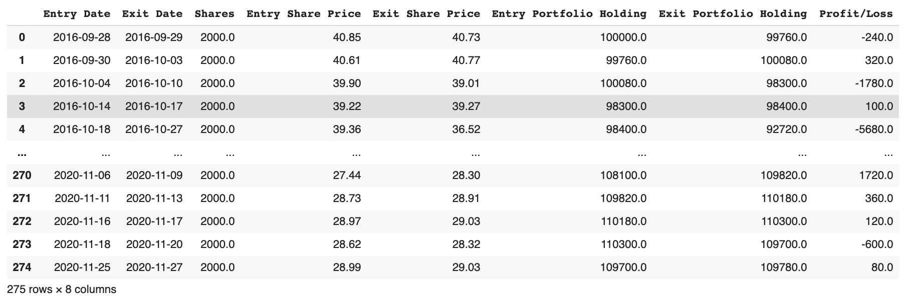
This allowed us to generate the following evaluation dataframe by feeding in the above-generated signals_df. It calculates important numbers such as Entry/Exit Share Prices and Profit/Loss, all per trade:
ANOVA tables were generated utilizing statsmodels' Ordinary Least Squares (OLS) model, a model analogous to Linear Regressions. The following is the ANOVA table generated for ATT's 3-Factor results:
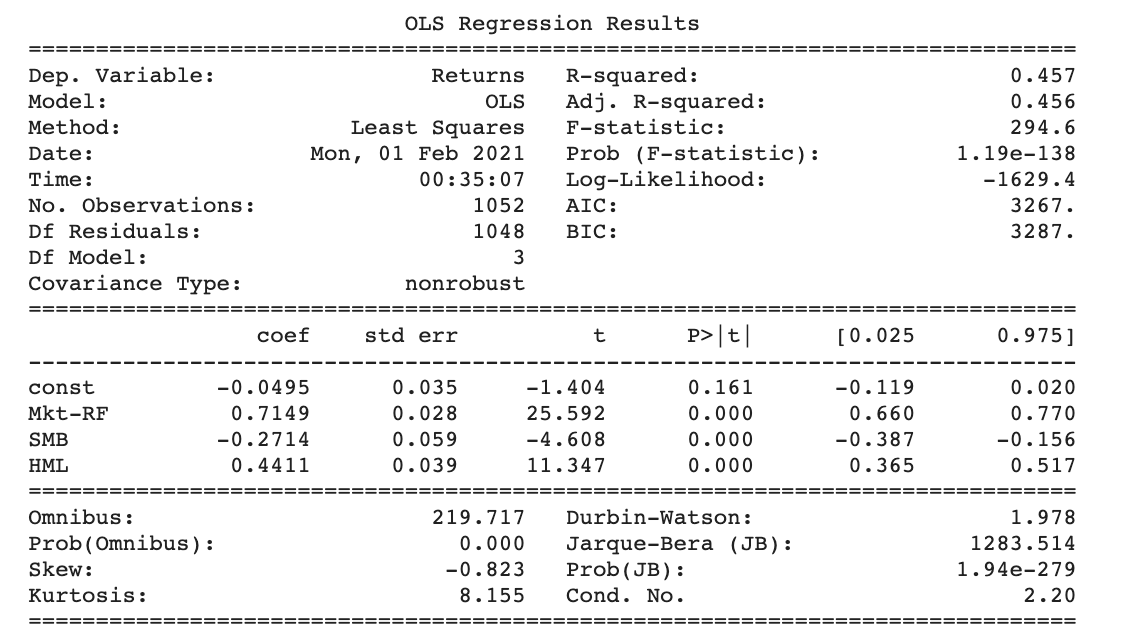
Few of the important numbers we'd like to point out: the first is R-squared. The way to read this is that 45.7% of the variation in y, which was excess return on the market, is explained by the factors. As there were only 3 factors, we expected to see that the 5 factor fama French model might yield better results.
The prob (f-statistic) depicts probability of the null hypothesis being true, and can be thought of as the p-value for the regression as a whole. Our f-statistic of near-0 implies that overall, the regressions were meaningful.
Last thing are the coefficients and the p-values for the X variables. The coefficients tell you the size of the effect that variable is having on the dependent variable, when all other independent variables are held constant. We can see out of all 3 variables, Mkt-Rf has the greatest impact on Returns, which makes intuitive sense as Mkt-Rf is directly used to calculate Returns. In regards to the p-values for the individual variables: these variables are correlated, and we see that a couple of the variables were deemed insignificant by the model, while the overall p-value was significant. We reasoned that this is because there is multicollinearity going on with the variables that are explaining the same part of the variation in returns, so their "significance" is divided up among them.
Seaborn Pair Plots were also generated for each stock. This plot shows the affect of all X variables when all of the other X variables are held constant. It acts as a visualization of the variable coefficients: the higher the coefficient, the more severe the slope of the line will be, either positively or negatively correlated. This is the Seaborn Pair Plot for ATT's Three-Factor model:
 With Mkt-Rf on the X-axis, we see that as it goes up so do returns, which makes sense, as it had the highest coeffiecient. The other two variables had slight effects on the dependent variable.
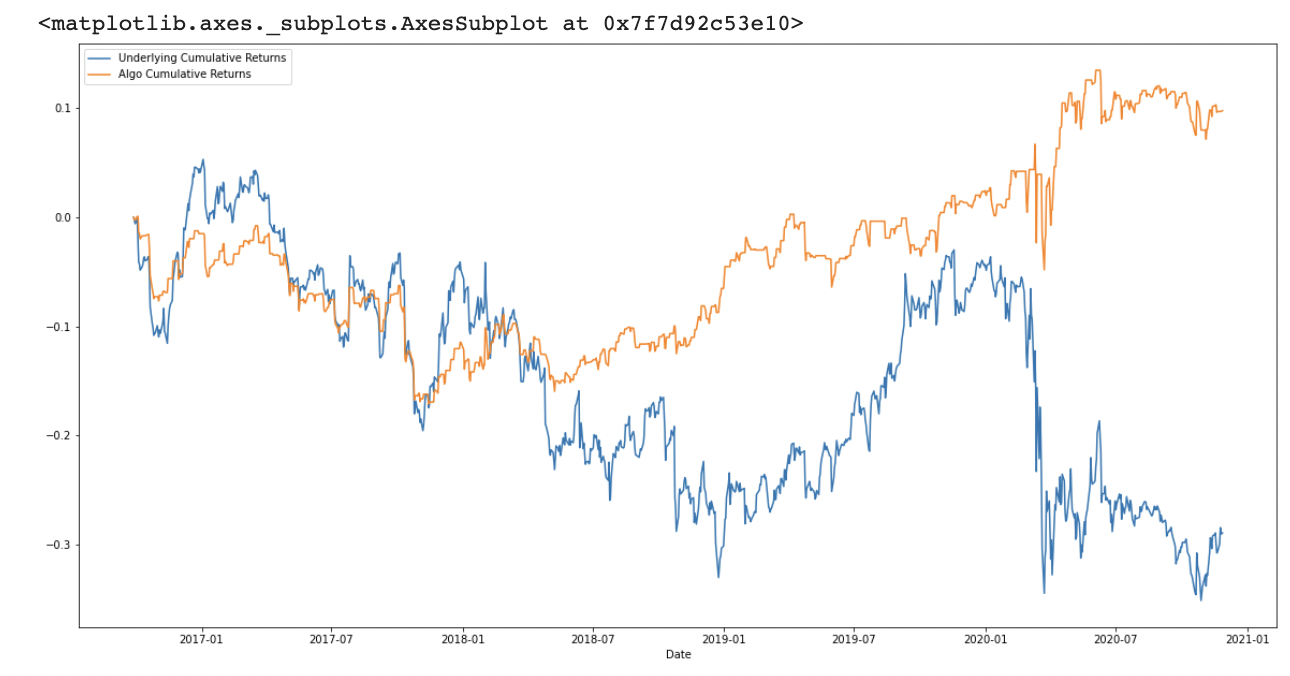
The above plot was generated for each stock analyzed: ATT, DIS and SPY, this one being for ATT. It is a visual representation of the 3-factor algorithm's cumulative returns vs. the underlying, aka buy-and-hold, return. We see in the above plot that for ATT, our backtested strategy signficantly outperformed a simple buy-and-hold strategy; while our backtested strategy had positive returns, if you were to buy-and-hold, you would have lost money.
Now it was time to do the same as we just did, but this time, using the Fama-French Five-Factor Model rather than the Three-Factor model. The 2 additional factors are RMW (Robust Minus Weak returns, aka the Profitability Factor) and CMA (Conservative Minus Aggressive returns, aka the Investment Factor). Given that there were 2 additional factors added for which the model could utilize to help make predictions, the group anticipated that these results would be significantly better than those we had observed for the Three-Factor model.
This is where our custom functions came in handy: we used our pre-defined functions to read-in the new Five-Factor dataframe and perform all the necessary calculations and evaluations. New code was not needed to be written. Therefore, we can jump straight to results for the Five-Factor Model:
Just like for the Three-Factor Model, ANOVA tables were generated utilizing statsmodels' Ordinary Least Squares (OLS) model, a model analogous to Linear Regressions. The following is the ANOVA table generated for ATT's 5-Factor results:

R-squared increased only slightly, from 45.7% to 47.3%, and the f-statistic was already near-0 with 3 factor. In terms of coefficients and individual p-values, Mkt-Rf remained the most influential variable, while the one of the new variables, RMW, was the 2nd most influential. Again, we saw multicollinearity among the X-variables. Overall, adding these 2 additional factors did not have a significant impact on the model.
 Similar to the Three-Factor model, we see that Mkt-Rf is the most influential stock in either direction, positive or negative. With more factors added, these charts were less steep than when there are only 3 factors because with more relevant factors added, each one now inherently has less of an effect on returns.

We see in the above plot that for ATT, our backtested strategy signficantly outperformed a simple buy-and-hold strategy; while our backtested strategy had positive returns, if you were to buy-and-hold, you would have lost money. Interestingly, total cumulative returns for the Five-Factor Model were less than those of the Three-Factor Model.
$T: 45.7% R-squared for 3-factor, 47.3% R-squared for 5-factor; .0978 Cumulative Return for 3-factor, .0688 Cumulative Return for 5-factor
$DIS: 51.2% R-squared for 3-factor, 52.2% R-squared for 5-factor; -.416 Cumulative Return for 3-factor, -.3166 Cumulative Return for 5-factor
$SPY: 99.3% R-squared for 3-factor, 99.3% R-squared for 5-factor; .5308 Cumulative Return for 3-factor, .4516 Cumulative Return for 5-factor
As the above shows, the 5-factor model did not always improve the model / increase our hypothetical, backtested returns. In terms of R-squared, the 5-factor model only slightly improved the values for ATT and Disney, and for SPY, it did not improve as it was already at 99.3%. In terms of the algorithm's cumulative returns, overall, adding the 2 additional factors actually decreased overall returns; only when the return was negative, like it was for $DIS, did adding the 2 additional factors benefit by decreasing overall loss.
This is not something that the group was necessarily surprised by, especiallly after doing our research and reading about what economists really thought about the validity of the 2 models. Ultimately, the 5-factor model still ignores momentum and volatility factors, 2 factors believed to have an important impact on a stock's price, and instead opts for adding profitability and investment factors (RMW and CMA, respectively). Many experts seem to question why these two particular factors were added to the 5-Factor model, and not a more appropriate set of variables; why stop at adding 2? Perhaps a next-step to this project would be to include these missing factors, momentum and volatility, and see if those factors are more reliable than profitability and investment factors.
In conclusion, we hope to have given a clear application of the Fama-French 3 and 5-Factor Model and how it can be applied to algorithmic trading / trading signals. Our results mirrored the findings of previous research in this area: the Fama-French 5-Factor model, although introducing 2 new factors that the 3-Factor Model does not have, is not necessarily a more effective model on which to make investment decisions.