CfC SageMaker Algorithm

The Time Series Forecasting (CfC) Algorithm from AWS Marketplace performs time series forecasting with the Closed-Form Continuous-Depth (CfC) network. It implements both training and inference from CSV data and supports both CPU and GPU instances. The training and inference Docker images were built by extending the PyTorch 2.1.0 Python 3.10 SageMaker containers. The Docker images include software licensed under the Apache License 2.0, see the attached LICENSE.

Model Description

The closed-form continuous-depth network (CfC) is a neural network architecture for sequential data. CfCs belong to the class of continuous-time recurrent neural networks (CT-RNN), where the evolution of the hidden state over time is described by an Ordinary Differential Equation (ODE).

CfCs use the Liquid Time Constant (LTC) ODE, where both the derivative and the time constant of the hidden state are determined by a neural network. Differently from other CT-RNNs (including LTCs), which use a numerical solver to approximate the ODE solution, CfCs use an approximate closed-form solution. As a results, CfCs achieve faster training and inference performance than other CT-RNNs.

The hidden state $x$ of a CfC at time $t$ is given by

$x(t) = \sigma(-f(x, I; \theta_f)t) \odot g(x, I; \theta_g) + [1 - \sigma(-[f(x, I; \theta_f)]t)] \odot h(x, I; \theta_h)$

where $\odot$ is the Hadamard product, $\sigma$ is the sigmoid function, $I$ is the input sequence, while $f$, $g$ and $h$ are neural networks. The three neural networks $f$, $g$ and $h$ share a common backbone, which is a stack of fully-connected layers with non-linear activation.

The backbone is followed by three separate neural network heads. The head of the $g$ and $h$ neural networks is a fully-connected layer with hyperbolic tangent activation. The head of the $f$ neural network is an affine function $b + a(\Delta t)$ where $\Delta t$ is the time span (or time increment) between consecutive time steps while the intercept $b$ and slope $a$ are the outputs of two fully-connected layers with linear activation.

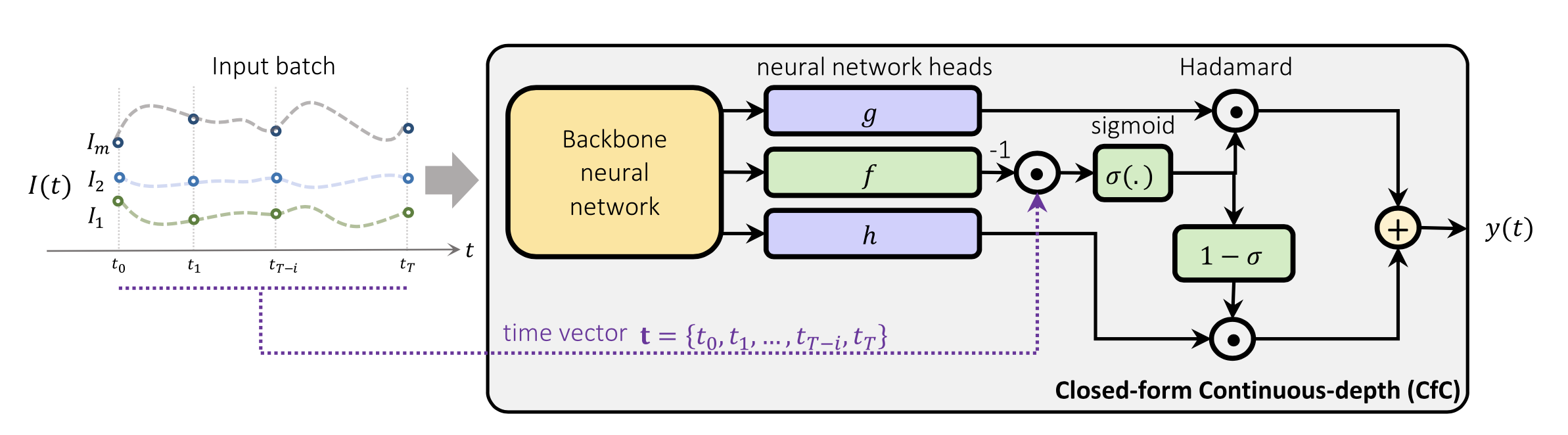
CfC architecture (source: doi:10.1038/s42256–022–00556–7)

Model Resources: [Paper] [Code]

SageMaker Algorithm Description

The algorithm implements the model as described above with no changes.

Training

The training algorithm has two input data channels: training and validation. The training channel is mandatory, while the validation channel is optional.

The training and validation datasets should be provided as CSV files. Each column represents a time series, while each row represents a time step. All the time series should have the same length and should not contain missing values. The column headers should be formatted as follows:

• The column names of the (mandatory) target time series should start with "y" (e.g. "y1", "y2", ...).
• The column names of the (optional) feature time series should start with "x" (e.g. "x1", "x2", ...).
• The column containing the time spans (optional) should be named "ts".

If the features are not provided, the algorithm will only use the past values of the target time series as input. If the time spans are not provided, the algorithm will assume that the observations are equally spaced. The time series are scaled internally by the algorithm, there is no need to scale the time series beforehand.

See the sample input files train.csv and valid.csv. See notebook.ipynb for an example of how to launch a training job.

Distributed Training

The algorithm supports multi-GPU training on a single instance, which is implemented through torch.nn.DataParallel. The algorithm does not support multi-node (or distributed) training across multiple instances.

Incremental Training

The algorithm supports incremental training. The model artifacts generated by a previous training job can be used to continue training the model on the same dataset or to fine-tune the model on a different dataset.

Hyperparameters

The training algorithm takes as input the following hyperparameters:

• context-length: int. The length of the input sequences.
• prediction-length: int. The length of the output sequences.
• sequence-stride: int. The period between consecutive output sequences.
• backbone-layers: int. The number of hidden layers of the backbone neural network.
• backbone-units: int. The number of hidden units of the backbone neural network.
• backbone-activation: str. The activation function of the backbone neural network.
• backbone-dropout: float. The dropout rate of the backbone neural network.
• hidden-size: int. The number of hidden units of the neural network heads.
• minimal: bool. If set to 1, the model will use the CfC direct solution.
• no-gate: bool. If set to 1, the model will use a CfC without the (1 - sigmoid) part.
• use-ltc: bool. If set to 1, the model will use an LTC instead of a CfC.
• use-mixed: bool. If set to 1, the model will mix the CfC RNN-state with an LSTM.
• lr: float. The learning rate used for training.
• lr-decay: float. The decay factor applied to the learning rate.
• batch-size: int. The batch size used for training.
• epochs: int. The number of training epochs.

Metrics

The training algorithm logs the following metrics:

• train_mse: float. Training mean squared error.
• train_mae: float. Training mean absolute error.

If the validation channel is provided, the training algorithm also logs the following additional metrics:

• valid_mse: float. Validation mean squared error.
• valid_mae: float. Validation mean absolute error.

See notebook.ipynb for an example of how to launch a hyperparameter tuning job.

Inference

The inference algorithm takes as input a CSV file containing the time series. The CSV file should have the same format and columns as the one used for training. See the sample input file test.csv.

The inference algorithm outputs the predicted values of the time series and the standard deviation of the predictions.

Notes:

a) The model predicts the time series sequence by sequence. For instance, if the context-length is set equal to 200, and the prediction-length is set equal to 100, then the first 200 data points (from 1 to 200) are used as input to predict the next 100 data points (from 201 to 300). As a result, the algorithm does not return the predicted values of the first 200 data points, which are set to missing in the output CSV file.

b) The outputs include the out-of-sample forecasts beyond the last time step of the inputs. For instance, if the number of input samples is 500, and the prediction-length is 100, then the output CSV file will contain 600 samples, where the last 100 samples are the out-of-sample forecasts.

See the sample output files batch_predictions.csv and real_time_predictions.csv. See notebook.ipynb for an example of how to launch a batch transform job.

Endpoints

The algorithm supports only real-time inference endpoints. The inference image is too large to be uploaded to a serverless inference endpoint.

See notebook.ipynb for an example of how to deploy the model to an endpoint, invoke the endpoint and process the response.

Additional Resources: [Sample Notebook] [Blog Post]

References

• R. Hasani, M. Lechner, A. Amini, D. Rus and R. Grosu, "Liquid time-constant networks", in Proceedings of the AAAI Conference on Artificial Intelligence, vol. 35, no. 9, pp. 7657-7666, 2021, doi: 10.1609/aaai.v35i9.16936.
• R. Hasani, M. Lechner, A. Amini, L. Liebenwein, A. Ray, M. Tschaikowski, G. Teschl and D. Rus, "Closed-form continuous-time neural networks", in Nature Machine Intelligence, vol. 4, pp. 992–1003, 2022, doi: 10.1038/s42256-022-00556-7.